Standard Costing Archives - EP Online Study

Standard Costing | Material Variance | Labour Variance | BQ | DQ | AQ

Manju@2050 — Fri, 11 Feb 2022 08:24:28 +0000

Standard Costing

Standard costing is pre-determined cost.

It is determined in advance of production like cost of materials, wages or labour, overheads etc.

It is a management accounting tools for management control.

It is applied to compare the actual cost with variance.

It is used for following process:

Establishment of standard cost

To find out actual cost

To compare and measurement of variance

Analysis of variances

Reporting to related center for taking action

Materials

In a manufacturing company, materials and labour are the most important factors for production.

Raw materials are converted into semi-finished goods and finished goods with the help of labour.

While manufacturing the goods, all the input goods are NOT output or yield.

There are normal and abnormal losses.

When the company cannot stop or control the loss of goods on a natural basis; it is called normal loss.

Normal losses are weight loss, shrinkage, evaporation, rust etc.

When the company can stop or control loss but could not control, it is known as abnormal loss.

Abnormal loss is due to carelessness, fatigue, rough handling, abnormal or bad working condition, lack of proper knowledge, low-quality raw materials, machine break down, accidents etc.

We will study the following materials variances in this topic:

Materials cost variance

Materials price variance

Materials usage variance

Materials mix variance

Materials yield variance

Click on the photo for FREE eBooks

Labour

Every manufacturing company and business organization needs human being resources.

These human beings may be the resource of administrators and labour.

Without labour, a manufacturing company cannot complete its production.

It is saying, “Talented, calibre and skilled manpower is the other assets of the business organization.”

There are three types of labour.

They are unskilled labour, semi-skilled labour and skilled labour.

Unskilled labour gets fewer wages but skilled labour gets the highest wages.

The payment made to the labour in exchange for its service is called labour cost.

It is a major part of the total cost of production.

Labour cost is also commonly called wages.

Labour cost or wages is one of the major elements of cost.

Labour cost represents the expense incurred on both direct and indirect labour.

Unproductive time is known as idle time.

It may be due to normal or abnormal reasons.

In idle time, workers have been paid without any production activity.

To identify the reasons for the idle time in the factory, an idle time card is maintained.

We will study the following labour variances in this topic:

Labour rate variance

Labour efficiency variance

Labour idle time variance

Labour mix variance

Labour yield variance

Labour cost variance

Brief Questions

Here, Amount = Rs = $ = £ = € = ₹ = Af = ৳ = Nu = Rf = රු = Br = P = Birr = Currency of your country

BQ: 1

Following data is available for materials X:

Standard rate of materials per kg	$40	Actual materials consumed	2,200 kg
Standard quality of materials	2,000 kg	Actual rate of materials per kg	$38
Standard rate of standard mix	$80,000	Actual rate of actual mix	$83,600

Required: (three variances of materials)

(a) Materials price variance; (b) Materials usage variance; (c) Materials cost variance

[Answer: MPV = $4,400 F; MUV = $8,000 U; MVC = $3,600 U]

Here, Amount = Rs = $ = £ = € = ₹ = Af = ৳ = Nu = Rf = රු = Br = P = Birr = Currency of your country

BQ: 2

The following data related to materials are given:

Standard materials mix			Actual materials mix
Materials	kg	Rate per kg	Materials	Units	Rate per kg
X	500	50	X	600	45

Required: (a) Materials price variance; (b) Materials usage variance; (c) Materials cost variance

[Answer: MPV = $3,000 F; MUV = $5,000 U; MCV = $2,000 U]

Here, Amount = Rs = $ = £ = € = ₹ = Af = ৳ = Nu = Rf = රු = Br = P = Birr = Currency of your country

BQ: 3

The following extracted data are given:

	Standard			Actual
Labour	No./mix	Rate ($)	Cost	No./mix	Rate($)	Cost
Trainee	1,000	25	25,000	1,100	22.50	24,750

Required: (a) Labour rate variance; (b) Labour efficiency variance; (c) Labour cost variance

[Answer: LRV = $2,750 F; LEV = $2,500 U; LCV = $250 F]

######

Click on the link for YouTube videos
Accounting Equation	http://tiny.cc/c89jkz
Journal Entries in Nepali	http://tiny.cc/uaakkz
Journal Entries	http://tiny.cc/8aakkz
Journal Entry and Ledger	http://tiny.cc/caakkz
Ledger	http://tiny.cc/haakkz
Subsidiary Book	http://tiny.cc/399jkz
Cashbook	http://tiny.cc/889jkz
Trial Balance and Adjusted Trial Balance	http://tiny.cc/c59jkz
Bank Reconciliation Statement (BRS)	http://tiny.cc/q59jkz
Depreciation	http://tiny.cc/ugakkz

Click on the link for YouTube videos chapter wise
Financial Accounting and Analysis (All videos)	http://tiny.cc/jlersz
Accounting Process	http://tiny.cc/mlersz
Accounting for Long Lived Assets	http://tiny.cc/plersz
Analysis of Financial Statement	http://tiny.cc/slersz

######

Descriptive Questions

Materials Variances

Here, Amount = Rs = $ = £ = € = ₹ = Af = ৳ = Nu = Rf = රු = Br = P = Birr = Currency of your country

DQ: 1

The following data related to materials are given:

Standard materials mix				Actual materials mix
Materials	Units	Rate	Amount	Materials	Units	Rate	Amount
A	600	15	9,000	A	500	24	12,000
B	200	35	7,000	B	100	60	6,000

There is not any loss during production.

Required: (a) Materials price variance; (b) Materials mix variance; (c) Materials usage variance; (d) Materials cost variance

[Answer: MPV = $7,000 U; MMV = $1,000 F; MUV = $5,000 F;

MCV = $2,000 U* SP₁ = 18.33; SP₂ = 20

Here, Amount = Rs = $ = £ = € = ₹ = Af = ৳ = Nu = Rf = රු = Br = P = Birr = Currency of your country

DQ: 2

The following data related to materials are given:

Standard materials mix			Actual materials mix
Materials	Kg	Rate	Materials	Kg	Rate
M	200	20	M	100	35
N	400	25	N	200	20
O	400	30	O	500	25

Standard and actual outputs were 1,000 units. Standard loss is 10% and actual output is 750 units.

Required: (a) Materials price variance; (b) Materials mix variance; (c) Materials yield variance; (d) Materials usage variance;

(e) Materials cost variance

[Answer: MPV = $2,000 F; MMV = $1,200 U;

MYV = $867 F; MUV = $333 U;

MCV = $1,667 F *SP₁ = 27.50; SP₂ = 26; SP₃ = 28.889

Here, Amount = Rs = $ = £ = € = ₹ = Af = ৳ = Nu = Rf = රු = Br = P = Birr = Currency of your country

DQ: 3

The standards cost for a product of the company shows the following materials standard:

Standard			Actual
Materials	Quantity	price per kg	Materials	Quantity	price per kg
A	4 kg	$5	A	150 kg	$4
B	1 kg	$10	B	40 kg	$10
C	5 kg	$20	C	210 kg	$25

The standard loss is 10% Actual output of the finished product is 380 kg.

Required: (1) (a) Material mixed variance; (b) Material yield variance; (c) Material price variance

(2) Write down any four advantages of standard costing

[Answer: MPV = $900 U; MMV = $150 U; MYV = ($287) F]

*SP₁= 13.375; SP₂ = 13; SP₃ = 14.44

Here, Amount = Rs = $ = £ = € = ₹ = Af = ৳ = Nu = Rf = රු = Br = P = Birr = Currency of your country

DQ: 4

The following details material standard and consumption have been provided

Materials	Standard			Actual
Materials	Quantity	Rate	Cost	Quantity	Rate	Cost
A	2	4	8	190	4.00	760
B	3	3	9	290	3.00	899
C	5	2	10	510	1.80	918
	10		$27	990		$2,577

Standard output 8 units and actual output 800 units

Required: (a) Material yield variance; (b) Materials mix variance; (c) Materials use variance; (d) Materials price variances

[Answer: MPV = ($73) F; MMV = ($23) F; MYV = ($27) F; MUV = ($50) F]

SP₁= 2.677; SP₂ = 2.7; SP₃ = 3.375

Here, Amount = Rs = $ = £ = € = ₹ = Af = ৳ = Nu = Rf = රු = Br = P = Birr = Currency of your country

DQ: 5

The details regarding materials are:

Materials	Standard			Material consumed
	Quantity in units	Price	Cost	Quantity in units	Price	Cost
A	30	$3	$90	280	$2.75	$770
B	30	$2	$60	265	$2.00	$530
C	40	$1	$40	375	$1.20	$450
	100		$190	920		$1,750

Standard loss 20% and Actual output 720 units

Required: (a) Material yield variance; (b) Materials mix variance; (c) Materials usage variance; (d) Materials price variances

[Answer: MPV = $5 U; MMV = ($3) F; MYV = $38 U; MUV = $35 U]

SP₁= 1.897; SP₂ = 1.9; SP₃ = 2.375

Labour Variances

Here, Amount = Rs = $ = £ = € = ₹ = Af = ৳ = Nu = Rf = රු = Br = P = Birr = Currency of your country

DQ: 6

The following extracted information is available:

Labour	Standard		Actual
Labour	No. of workers	Wage rate per hour	No. of workers	Wage rate per hour
Semi -skilled	200	$37.50	220	$36.00
Unskilled	100	$22.50	80	$24.00

Standard time fixed for work 50 hours. Work actually completed in also 50 hours.

Required: (Direct) (a) Labour rate variance; (b) Labour mix variance; (c) Labour efficiency variance; (d) Labour cost variances

[Answer: LRV = $10,500 F; LMV = $15,000 U; LEV = $15,000 U;

LCV = $4,500 U] *SR₁ = 10,050; SR₂ = 9,750;

Here, Amount = Rs = $ = £ = € = ₹ = Af = ৳ = Nu = Rf = රු = Br = P = Birr = Currency of your country

DQ: 7

ABC Company gives you following standard and actual data:

Standard				Actual
Workers	No.	Rate per hour	Hours worked	Workers	No.	Rate per hour	Hours Worked
Grade A	50	$50	100	Grade A	30	$75	120
Grade B	100	$25	100	Grade B	120	$20	120

Required: (a) Labour mix variance; (b) Labour efficiency variance; (c) Labour rate variance; (d) Labour yield variance

[Answer: LRV = $18,000 U; LMV = ($60,000) F; LYV = $100,000 U;

LEV = $40,000 U] *SR₁ = 4500; SR₂ = 5000;

Here, Amount = Rs = $ = £ = € = ₹ = Af = ৳ = Nu = Rf = රු = Br = P = Birr = Currency of your country

DQ: 8

The following extracted data related to labour of ABC Company has given below:

Standard			Actual
Labour	Hour per unit	Rate per hour	Labour	Hours per unit	Rate per hour
Skilled	5	37.50	Skilled	4.5	50.00
Semi-skilled	4	18.75	Semi-skilled	4.2	18.75
Unskilled	8	12.50	Unskilled	10	11.25

Standard and actual productions were 1,000 units. Standard and actual gang time 48 hours in a week.

Required: (Direct): (a) Labour rate variance; (b) Labour mix variance; (c) Labour yield variance; (d) Labour efficiency variance;

(d) Labour cost variances

[Answer: LRV = $2,100 U; LMV = $480 U; LYV = Nil; LEV = $480 U;

LCV = $2,580 U; *SR₁ = 372.5; SR₂ = 362.5; SR₃ = 17.40

Here, Amount = Rs = $ = £ = € = ₹ = Af = ৳ = Nu = Rf = රු = Br = P = Birr = Currency of your country

DQ: 9

The details regarding labor cost have been provided as:

Type	Standard			Actual
Type	No.	Rate/Hour	Cost	No.	Rate/Hour	Cost
Skilled	1	$50	50	1	$45	45
Semi- skilled	3	$30	90	4	$30	120
Unskilled	6	$20	120	5	$22	110
	10		260	10		275

40 hours a week needed to work and paid. Actual output produced 360 units. Standard output per gang hour is 8 units.

Required: (direct): (a) Labour rate variance; (b) Labour mix variance; (c) Labour efficiency sub (yield) variance;

(d) Labour efficiency variance; (e) Labour cost variance

[Answer: LRV = $200 U; LMV = $400 U; LYV = ($1,300) F; LEV = ($900) F;

LCV = ($700) F] *SR₁ = 270; SR₂ = 260; SR₃ = 32.5

Click on the photo for FREE eBooks

ACCOUNTING, ECONOMICS, BUSINESS STUDIES, FINANCE, ENGLISH eBooks, EP Online Study

Analytical Questions

Here, Amount = Rs = $ = £ = € = ₹ = Af = ৳ = Nu = Rf = රු = Br = P = Birr = Currency of your country

AQ: 1

ABC Manufacturing Company provides you following information related to materials.

Standard materials cost with 1 ton output were:		Actual materials cost with 1,000 kg output were:
Materials A	300 kg at $100	Materials A	0.35 tons at $90,000 per ton
Materials B	400 kg at $50	Materials B	0.42 tons at $60,000 per ton
Materials C	500 kg at $60	Materials C	0.53 tons at $70,000 per ton

Required: (a) Materials price variance; (b) Materials mix variance; (c) Materials yield variance; (d) Materials usage variance;

(e) Materials cost variance

MPV = $6,000 U; MPV = $1,113 U; MYV = $6,667 U;

MUV = $7,800 U; MCV = $13,800 U]

* 1 ton = 1,000 kg] *SP₁ = 67.538; SP₂ = 66.667; SP₃ = 80

Here, Amount = Rs = $ = £ = € = ₹ = Af = ৳ = Nu = Rf = රු = Br = P = Birr = Currency of your country

AQ: 2

XYZ Company (P) Ltd has information:

Standard			Actual
Labour	No./mix	Rate ($)	Labour	No./mix	Rate ($)
Skilled	10	50	Skilled	13	48
Semi-skilled	5	32	Semi-skilled	4	34
Unskilled	5	28	Unskilled	3	26
Total	20		Total	20
Normal working hours (STG) 40 hours			Actual output realized 960 hours
Standard output 1,000			Abnormal idle time 2 hours

Required: (a) Labour rate variance; (b) Labour ideal time variance; (c) Labour mix variance; (d) Labour yield variance;

(e) Labour efficiency variance; (f) Labour cost variance

[Answer: LRV = ($960) F; LITV = $1,724 U; LMV = $2,356 U;

LYV = ($320) F; LEV = $3,760 U; LCV = $2,800 U]

*SR₁ = 862; SR₂ = 800; SR₃ = 32

Here, Amount = Rs = $ = £ = € = ₹ = Af = ৳ = Nu = Rf = රු = Br = P = Birr = Currency of your country

AQ: 3

APD Power (P) Ltd has following labour data:

Standard			Actual
Labour	No.	Rate per hour ($)	Labour	No.	Rate per hour ($)
Grade A	30	48	Grade A	40	42.00
Grade B	15	36	Grade B	10	40.80
Grade C	10	24	Grade C	5	18.00

Normal working hours in week is 40 hours. Standard yield was 1,600 units. It is expected to produce by gang 2,000 hours during the period but actual yield was 1,980 hours due to four abnormal idle times.

Required: (a) Labour rate variance; (b) Labour ideal time variance; (c) Labour mix variance; (d) Labour yield variance;

(e) Labour efficiency variance; (f) Labour cost variance

[Answer: LRV = ($8,880) F; LITV = $2,400 U; LMV = $7,020 U;

LEV = ($23,310) F; LEV = ($13,890) F; LCV = ($22,770) F]

[Answer: LRV = ($4,040) F; LITV = $1,200 U; LMV = $3,510 U;

LYV = ($11,655) F; LEV = ($6,945) F; LCV = ($11,385) F]

*SR₁ = 2,400; SR₂ = 2,220; SR₃ = 55.50

Here, Amount = Rs = $ = £ = € = ₹ = Af = ৳ = Nu = Rf = රු = Br = P = Birr = Currency of your country

AQ: 4

ABC Manufacturing Company has following data related to materials and labour:

Standard			Actual
Kg	Materials	Rate	Kg	Materials	Rate
450	A	20	450	A	19
360	B	10	360	B	11

Hours	Labour	Rate	Hours	Labour	Rate
2,400	Skilled	40	2,400	Skilled	45
1,200	Unskilled	20	1,200	Unskilled	25

For materials as well as labour, standard loss is 90 kg and actual yield is 760 kg.

Required: (Direct)

Materials price variance	Labour rate variance
Materials mix variance	Labour mix variance
Materials yield variance	Labour yield variance
Materials efficiency/usage variance	Labour efficiency/use
Materials cost variance	Labour cost variance

[Answer for materials: MPV = ($90) U; MMV = Nil; MYV = ($700) F;

MUV = ($700) F; MCV = ($790) F]

SP₁ = 15.556; SP₂ = 15.556; SP₃ = 17.5

[Answer for labour: LRV = $18,000 U; LMV = Nil; LYV = ($6,669) F;

LEV = ($6,669) F; LCV = $11,331 U]

SR₁ = 120,000; SR₂ = 120,000; SR₃ = 166.67

EP Online Study

Thank you for investing your time.

Please comment on the article and share this post on your social media platform.

Jay Google, Jay YouTube, Jay Social Media

जय गूगल. जय युट्युब, जय सोशल मीडिया

Labour Variance | Rate | Efficiency | Idle Time | Mix | Yield | Cost | Problem & Solution

Manju@2050 — Fri, 11 Feb 2022 06:13:08 +0000

Materials

In a manufacturing company, materials and labour are the most important factors for production.

Raw materials are converted into semi-finished goods and finished goods with the help of labour.

While manufacturing the goods, all the input goods are NOT output or yield.

There are normal and abnormal losses.

When the company cannot stop or control the loss of goods on a natural basis; it is called normal loss.

Normal losses are weight loss, shrinkage, evaporation, rust etc.

When the company can stop or control loss but could not control, it is known as abnormal loss.

Abnormal loss is due to carelessness, fatigue, rough handling, abnormal or bad working condition, lack of proper knowledge, low-quality raw materials, machine break down, accidents etc.

We will study the following materials variances in this topic:

Materials cost variance

Materials price variance

Materials usage variance

Materials mix variance

Materials yield variance

Click on the photo for FREE eBooks

Labour

Every manufacturing company and business organization needs human being resources.

These human beings may be the resource of administrators and labour.

Without labour, a manufacturing company cannot complete its production.

It is saying, “Talented, calibre and skilled manpower is the other assets of the business organization.”

There are three types of labour.

They are unskilled labour, semi-skilled labour and skilled labour.

Unskilled labour gets fewer wages but skilled labour gets the highest wages.

The payment made to the labour in exchange for its service is called labour cost.

It is a major part of the total cost of production.

Labour cost is also commonly called wages.

Labour cost or wages is one of the major elements of cost.

Labour cost represents the expense incurred on both direct and indirect labour.

Unproductive time is known as idle time.

It may be due to normal or abnormal reasons.

In idle time, workers have been paid without any production activity.

To identify the reasons for the idle time in the factory, an idle time card is maintained.

We will study the following labour variances in this topic:

Labour rate variance

Labour efficiency variance

Labour idle time variance

Labour mix variance

Labour yield variance

Labour cost variance

Direct Labour Variance | Labour Variance

Every production company needs labour for production.

By using the labour, the company produces goods.

While producing the goods, there may be variances.

A labour variance arises when the actual cost varies from expected budgeted or standard amount.

This varies either better or worse.

The difference between standard cost of labour and actual cost of labour is labour/wage variance.

Direct labour cost variance is the difference between the standard cost for actual production and the actual cost in production.

There are two kinds of labour variances.

They are labour rate variance and labour efficiency variance.

Labour rate variance is the difference between the standard cost and the actual cost paid for the actual number of hours.

Labour efficiency variance is the difference between the standard labour hours.

The principle of labour cost variance is similar to materials cost variance.

Purchase of materials, usage of materials and usage of labour are connected with each other.

Before finding out labour variances, the following point should be found out (requirement for labour variance):

AR	= Actual wage rate per period (hour, day, week, month)
AT or AQ	= Actual time taken or actual quantity used for production
SR	= Standard wage rate per period (hour, day, week, month)
ST or SQ	= Standard time or standard quantity used for production
SY or SO	= Standard yield or output
AY or AO	= Actual yield or output
RSY	= Revised standard yield
IT	= Idle time
AGT	= Actual gang time
SGT	= Standard gang time
SR₁	= standard rate per unit of actual mix
SR₂	= standard rate per unit of standard mix
SR₃	= standard rate

Types of labour variance
Labour Rate Variance (LRV)
Labour Efficiency Variance (LEV)
Labour Idle Time Variance (LITV)
Labour Mix Variance (LMV)
Labour Yield Variance (LYV)
Labour Cost Variance (LCV)

(1) Labour cost variance, LCV

The difference between standard direct labour cost for actual activity and direct labour cost paid is known as direct labour cost variance.

LCV	= (Standard time × Standard rate) – (Actual time × Actual rate)
Or	= (ST × SR) – (AT × AR)

(2) Labour rate variance, LRV

The difference between standard wage rates fixed and actual wage paid as known labour rate variance.

LRV	= Actual time × (Standard rate – Actual rate)
Or	= AT × (SR – AR)

(3) Labour efficiency variance, LEV

The difference between labour hours specified for the activity achieved and actual labour hour expended as known labour efficiency variance.

LEV	= Standard rate × (Standard time – Actual time)
Or	= SR × (ST – AT)

Three (3) variances without mix and yield variances

Computation:	Variances:	by table	by formula
L₁= AT × AR	Labour Rate Variance (LVR)	= L₁ – L₂	= AT (SR– AR)
L₂= AT × SR	Labour Efficiency Variance (LEV)	= L₂ – L₃	= SR (ST– AT)
L₃= ST × SR	Labour Cost Variance (LCV)	= L₁ – L₃	= (ST × SR) – (AT × AR)

Here, Amount = Rs = $ = £ = € = ₹ = Af = ৳ = Nu = Rf = රු = Br = P = Birr = Currency of your country

PROBLEM: 2A

The following data related to labour are given below by HP Company (P) Ltd:

Standard labour mix			Actual labour mix
Labour	Hours/No.	Rate per hour	Labour	Hours/No.	Rate per hour
Skilled	200	$50	Skilled	150	$60

Required: (1) Labour rate variance; (2) Labour efficiency variance; (3) Labour cost variance

[Answer: LRV = $(1,500) U; LEV = $2,500 F; LCV = $1,000 F]

SOLUTION:

By table method:

Given and working note:

Labour	Standard			Actual			Standard × Actual
	No. (ST)	Rate (SR)	Amount	No. (AT)	Rate (AR)	Amount	SR × AT
Skilled	200	50	10,000	150	60	9,000	50 × 150 = 7,500
Total	200		SR₂ =10,000	150		9,000	SR₁ = 7,500

Again,

L₁= AT × AR = 150 × 60 = $9,000

L₂= AT × SR = 150 × 50 = $7,500

L₃= ST × SR = 200 × 50 = $10,000

Now,

Labour Rate Variance (LRV)	= L₁ – L₂	= 9,000 – 7,500	= $1,500 U
Labour Efficiency Variance (LEV)	= L₂ – L₃	= 7,500 – 10,000	= $(2,500) F
Labour Cost Variance(LCV)	= L₁ – L₃	= 9,000 – 10,000	= $(1,000) F

By formula method:

Labour rate variance (LRV)

= Actual time × (Standard rate – Actual rate)

= AT × (SR – AR)

= 150 (50 – 60)

= 150 × – 10

= ($1,500) U

Labour Efficiency Variance (LEV)

= Standard rate × (Standard time – Actual time)

= SR × (ST – AT)

= 50 × (200 – 150)

= 50 × 50

= $2,500 F

Labour cost variance (LCV)

= (Standard time × Standard rate) – (Actual time × Actual rate)

= (ST × SR) – (AT × AR)

= (200 × 50) – (150 × 60)

= 10,000 – 1,000

= $1,000 F

Keep in Mind (KIM)

Formula method

Table method

Positive result or answer means favorable (F)

Negative result or answer means un-favourable (U) or adverse (A)

Positive result or answer means unfavourable (U) or adverse (A)

Negative result or answer means favourable (F)

(4) Labour idle time variance, LITV

Labour idle time arises is due to abnormal wastage of time like strike, lock out, power failure, machinery break down etc.

Idle time variance is always adverse (unfavorable).

It is needed investigation for its causes.

It shows in-efficiency of workers although they are not responsible for this.

LITV	= Idle time × Standard rate
Or	= IT × SR

Four (4) variances without mix and yield variances

Computation:	Variances:	by table	by formula
L₁= AT × AR	Labour Rate Variance (LRV)	= L₁ – L₂	= AT × (SR– AR)
L₂ = AT × SR	Labour Ideal Time Variance (LITV)	= L₂ – L₃	= SR × IT
L₃ = (AT – IT) SR	Labour Efficiency Variance (LEV)	= L₃ – L₄	= SR × (ST– AT)
L₄ = ST × SR	Labour Cost Variance (LCV)	= L₁ – L₄	= (ST × SR) – (AT × AR)

Keep in Mind (KIM)

Labour idle time variance is always unfavourable either positive or negative answer

######

Click on the link for YouTube videos
Accounting Equation	http://tiny.cc/c89jkz
Journal Entries in Nepali	http://tiny.cc/uaakkz
Journal Entries	http://tiny.cc/8aakkz
Journal Entry and Ledger	http://tiny.cc/caakkz
Ledger	http://tiny.cc/haakkz
Subsidiary Book	http://tiny.cc/399jkz
Cashbook	http://tiny.cc/889jkz
Trial Balance and Adjusted Trial Balance	http://tiny.cc/c59jkz
Bank Reconciliation Statement (BRS)	http://tiny.cc/q59jkz
Depreciation	http://tiny.cc/ugakkz

Click on the link for YouTube videos chapter wise
Financial Accounting and Analysis (All videos)	http://tiny.cc/jlersz
Accounting Process	http://tiny.cc/mlersz
Accounting for Long Lived Assets	http://tiny.cc/plersz
Analysis of Financial Statement	http://tiny.cc/slersz

######

Here, Amount = Rs = $ = £ = € = ₹ = Af = ৳ = Nu = Rf = රු = Br = P = Birr = Currency of your country

PROBLEM: 2B

The following data related to labour are given below by ABC Manufacturing Company:

Standard labour mix			Actual labour mix
Labour	Hours/No.	Rate per hour	Labour	Hours/No.	Rate per hour
Unskilled	1,920	$24	Skilled	2,000	$27

Additional information:

Due to power failed of machinery, 20% of actual hours were idle time.

Standard time was 40 hours in a week.

Required: (a) Labour Rate Variance (LRV); (b) Labour Ideal Time Variance (LITV); (c) Labour Efficiency Variance (LEV);

(d) Labour Cost Variance (LCV)

[Answer: LVR = $6,000 U; LITV = $9,600 U;

LEV = $7,680 F; LCV = $7,920 U]

SOLUTION:

By table method:

Given and working note:

Labour	Standard			Actual			Standard × Actual
	SN	SR	Amount	AN	AR	Amount	SR × AT
Unskilled	1,920	24	46,080	2,000	27	54,000	24 × 2,000 = 48,000
Total	1,920		SR₂ = 46,080	2,000		ATR= 54,000	SR₁ = 48,000

Others

Standard gang time (SGT) = 40* hours

Actual gang time (AGT) = 40* hours

Idle time [2,000@20%] = 400 hours

Actual yield or output (AY) [2,000 –400] = 1,600

Again,

L₁	= AT × AR	= 2,000 × 27	= $54,000
L₂	= AT × SR	= 2,000 × 24	= $48,000
L₃	= (AT – IT) × SR	= (2,000 – 400) × 24	= $38,400
L₄	= ST × SR	= 1,920 × 24	= $46,080

Now,

Labour Rate Variance (LRV)	= L₁ – L₂	= 54,000 – 48,000	= 6,000 U
Labour Idle Time Variance (LITV)	= L₂ – L₃	= 48,000 – 38,400	= 9,600 U
Labour Efficiency Variance (LEV)	= L₃ – L₄	= 38,400 – 46,080	= (7,680) F
Labour Cost Variance (LCV)	= L₁– L₄	= 54,000 – 46,080	= 7,920 U

By formula method:

Labour rate variance (LRV)

= Actual time × (Standard rate – Actual rate)

= AT × (SR – AR)

= 2,000 × (24 – 27)

= 2,000 × – 3

= $(6,000) U

Labour Idle Time Variance (LITV)

Idle time = 2,000 hours @ 20% = 400 hours

= Idle time × Standard rate

= IT × SR

= 400 hours × $24

= $9,600 U

Labour Efficiency Variance (LEV)

= Standard rate × (Standard time – Actual time)

= SR × (ST – AT)

= 24 × (1,920 – 1,600)

= 24 × 320

= $7,680 F

Labour cost variance (LCV)

= (Standard time × Standard rate) – (Actual time × Actual rate)

= (ST × SR) – (AT × AR)

= (1,920 × 24) – (2,000 × 27)

= 46,080 – 54,000

= $(7,920) U

Keep in Mind (KIM)

Idle time variance always unfavourable or adverse for factory.

In efficiency variance, actual time (AT) is taken after deducting idle time.

(5) Labour mix variance LMV | Gang composition variance, GCV

The difference between standard labour grade and actual labour grade are known as labour mix variance.

There may be difference types of labour in the company.

They are unskilled labour, semi-skilled labour, skilled labour and highly skilled labour etc.

Their mix in the work is known gang composition, labour mix variance or gang composition variance.

There are different rules for labour mix variances.

When standard number of labour and actual number of labour is equal:

LMV = Standard rate × (Revised standard time – Actual time)

Where:

Revised standard time = Standard time × (Actual yield ÷ Standard yield)

When standard number of labour and actual number of labour is not equal:

LITV	= Idle time × Standard rate
	= IT × SR
	Or
LMV	[(Actual mix ÷ Standard mix) × Standard rate of standard mix] – (Standard rate of actual mix)
	[(ΣAT ÷ ΣST) × SR × ST] – (SR × AT)

Where:

ST = standard time = Standard labour No. × Standard gang time

AT = actual time = Actual labour No. × Actual gang time

ΣAT = Total of AT = total of Actual labour No. × Actual gang time

ΣST = Total of ST = total of Standard labour No. × Standard gang time

(6) Labour yield variance, LYV | Labour output variance, LOV

The difference between actual output of the workers and standard output of the workers are known as labour yield variance.

It can be also found out by the difference between labour mix variance and labour idle time variance.

When actual mix (number) and standard mix (number) are not vary or difference: (when idle time is not given)

LYV	= Standard cost per unit × (Actual yield or output – Standard yield for actual input)
Or	= SC × (AY – SY)

Standard cost

= Standard No. × Standard rate × Standard gang time

= SN × SR × SGT

Standard cost per unit (SC)

= Total standard cost ÷ Standard yield = (SR₂ × SGT) ÷ Standard yield = SR₃

When actual mix (number) and standard mix (number) are vary or difference: (when idle time is given)

LYV	= Standard cost per unit × (Actual yield or output – Revised standard yield or output)
Or	= SC × (AY – RSY)

Revised actual time (RAT)

= Actual Number (Standard gang time – Idle time)

= AN (SGT – IT)

Revised standard yield

= SY × ΣRAT ÷ ΣST

Four (4) variances with mix variance but without ideal time

Computation:		Standard rate per unit (SR₁, SR₂)
L₁= AGT × ATR		SR₁= standard rate per unit of actual mix
L₂= AGT × SR₁		SR₂= standard rate per unit of standard mix
L₃= AGT × SR₂
L₄= SGT or AY* × SR₂

Variances:	by table		by formula
Labour Rate Variance (LRV)	= L₁ – L₂		= AT × (SR – AR)
Labour Mix Variance (LMV)	= L₂ – L₃		= [ΣAT ÷ ΣST × SR × ST] – (SR × AT)
Labour Efficiency Variance (LEV)	= L₃ – L₄		= SR (ST – AT)
Labour Cost Variance(LCV)	= L₁ – L₄		= (ST × SR) – (AT × AR)

**If actual yield is not given in the question, standard gang time (SGT) is taken***

Keep in Mind (KIM)

If there are different between standard number of workers and actual number of workers, answer of mix variance and yield variance are different in table method and formula method.

Gang composition means labour mix variance.

Here, Amount = Rs = $ = £ = € = ₹ = Af = ৳ = Nu = Rf = රු = Br = P = Birr = Currency of your country

PROBLEM: 2C

The following data related to labour are given below MN Manufacturing Company:

Standard gang time was 30 hours but actual gang was 32 hours.

Standard labour mix			Actual labour mix
Labour	No.	Rate per hour ($)	Labour	No.	Rate per hour ($)
Men	100	60	Men	80	65
Women	40	36	Women	50	40
Boys	60	24	Boys	70	20

Required: (a) Labour Rate Variance (LRV); (b) Labour Mix Variance (LMV); (c) Labour Efficiency Variance (LEV);

(d) Labour Cost Variance (LCV)

[Answer: LRV = 10,240 U; LMV = 19,200 F; LEV = 1,440 F; LCV = $8,800 U]

SOLUTION:

By table method

Given and working note:

Labour	Standard			Actual			Standard × Actual
	SN	SR	Amount	AN	AR	Amount	SR × AN
Men	100	60	6,000	80	65	5,200	60 × 80 = 4,800
Women	40	36	1,440	50	40	2,000	36 × 50 = 1,800
Boys	60	24	1,440	70	20	1,400	24 × 70 = 1,680
Total			SR₂ = 8,880			ATR = 8,600	SR₁ = 8,280

Others

Standard gang time (SGT) = 30* hours

Standard output or yield =?

Actual gang time (AGT) = 32 hours

Actual output or yield =?

SR₁= standard rate in actual mix = $8,280

SR₂ = standard rate in standard mix = $8,880

Again

L₁= AGT × ATR	= 32 × 8,600	= $275,200
L₂= AGT × SR₁	= 32 × 8,280	= $264,960
L₃= AGT × SR₂	= 32 × 8,880	= $284,160
L₄= AY × SR₂ or [SGT × SR₂]*	= 30 × 8,880	= $266,400

Keep in Mind (KIM)

If actual yield (AY) is not given, standard gang time (SGT) is taken.

Now,

Labour Rate Variance (LRV)	= L₁ – L₂	= 275,200 – 264,960	= 10,240 U
Labour Mix Variance (LMV)	= L₂ – L₃	= 264,960 – 284,160	= (19,200) F
Labour Efficiency Variance (LEV)	= L₂ – L₄	= 264,960 – 266,400	= (1,440) F
Labour Cost Variance (LCV)	= L₁ – L₄	= 275,200 – 266,400	= 8,800 U

By formula method:

Given and working note:

Labour	Standard				Actual
	SN	SR	SGT	ST = SN × SGT	AN	AR	AGT	AT = AN × AGT
Men	100	60	30	3,000	80	65	32	2,560
Women	40	36	30	1,200	50	40	32	1,600
Boys	60	24	30	1,800	70	20	32	2,240
Total	200			ΣST = 6,000	200			ΣAT = 6,400

Labour rate variance (LRV)

LRV	= AT (SR – AR)
Men	= 2,560 (60 – 65)	= 2,560 × – 5	= (12,800) U
Women	= 1,600 (36 – 40)	= 1,600 × – 4	= (6,400) U
Boys	= 2,240 (24 – 20)	= 2,240 × 4	= 8,960 F
Total			= $10,240 U

Labour mix variance (LMV)

LMV	= [(ΣAT ÷ ΣST) × SR × ST] – (SR × AT)
Men	= [(6,400 ÷ 6,000) × 60 × 3,000] – (60 × 2,560)	= 192,000 – 153,600	= 38,400 F
Women	= [(6,400 ÷ 6,000) × 36 × 1,200] – (36 × 1,600)	= 46,080 – 57,600	= (11,520) U
Boys	= [(6,400 ÷ 6,000) × 24 × 1,800] – (24 × 2,240)	= 46,080 – 53,760	= (7,680) U
Total			= $19,200 F

Labour Efficiency Variance (LEV)

LEV	= Standard rate × (Standard time – Actual time)
	= SR × (ST – AT)
Men	= 60 × (3,000 – 2,560)	= 60 × 440	= 26,400 F
Women	= 36 × (1,200 – 1,600)	= 36 × – 400	= (14,400) U
Boys	= 24 × (1,800 – 2,240)	= 24 × – 440	= (10,560) U
Total			= $1,440 F

Labour cost variance (LCV)

LCV	= (Standard time × Standard rate) – (Actual time × Actual rate)
	= (ST × SR) – (AT × AR)
Men	= (3,000 × 60) – (2,560 × 65)	= 180,000 – 166,400	= 13,600 F
Women	= (1,200 × 36) – (1,600 × 40)	= 43,200 – 64,000	= (20,800) U
Boys	= (1,800 × 24) – (2,240 × 20)	= 43,200 – 44,800	= (1,600) U
Total			= $(8,800) U

Here, Amount = Rs = $ = £ = € = ₹ = Af = ৳ = Nu = Rf = රු = Br = P = Birr = Currency of your country

PROBLEM: 2D

The following data related to labour are given by ABC Small industries:

Labour	Standard labour mix		Actual labour mix
	No.	Rate per hour ($)	Labour	No.	Rate per hour ($)
Grade A	12	22.50	Grade A	15	20.00
Grade B	8	17.50	Grade B	6	18.75
Grade C	4	12.50	Grade C	5	10.00

Additional information:

In a normal working week of 48 hours, the gang expected to produce 1,200 units. In same working hours, actual output produced 1,000 units due to abnormal idle time of 8 hours.

Required: (a) Labour Rate Variance (LRV); (b) Labour Idle Time Variance (LITV); (c) Labour Mix Variance (LMV);

(d) Labour Yield Variance (LYV); (e) Labour Efficiency Variance (LEV); (f) Labour Cost Variance (LCV)

[Answer: LRV = (2,040) F; LITV = 4,040 U; LMV = (1,800) F;

LYV = Nil; LEV = 5,840 F; LCV = 3,800 U]

SOLUTION:

By table method

Given and working note:

Labour	Standard			Actual			Standard × Actual
	SN	SR	Amount	AN	AR	Amount	SR × AN
Grade A	12	22.50	270	15	20.00	300.00	22.50 × 15 = 337.50
Grade B	8	17.50	140	6	18.75	112.50	17.50 × 6 = 105.00
Grade C	4	12.50	50	5	10.00	50.00	12.50 × 5 = 62.50
Total			SR₂ = 460			ATR = 462.5	SR₁ = 505

Others

Standard gang time (SGT) = 48 *hours

Standard output per gang?

Standard yield (SY) (given) = 1,200 units

Actual gang time (AGT) = 48* hours

Idle time = 8 hours

Actual yield (AY) (given) = 1,000 units

Note: lack of information, standard gang hours and actual gang hours is same.

SR₁= standard rate in actual mix = $505

SR₂ = standard rate in standard mix = $460

SR₃ = standard rate in standard output = STG × SR2 ÷ Standard yield = 48 × 460 ÷ 1,200 = $18.4

Again

L₁= AGT × ATR	= 48 × 462.5	= $22,200
L₂= AGT × SR₁	= 48 × 505	= $24,240
L₃= (AGT – IT) × SR₁	= (48 – 8) × 505	= $20,200
L₄= (AGT – IT) × SR₂	= (48 – 8) × 460	= $18,400
L₄= AY × SR₃	= 1,000 × 18.4	= $18,400

Now,

Labour Rate Variance (LRV)	= L₁ – L₂	= 22,200 – 24,240	= (2,040) F
Labour Idle Time Variance (LITV)	= L₂ – L₃	= 24,240 – 20,200	= 4,040 U
Labour Mix Variance (LMV)	= L₃ – L₄	= 20,200 – 18,400	= 1,800 U
Labour Yield Variance (LYV)	= L₄ – L₅	= 18,400 – 18,400	= Nil (No variance)
Labour Efficiency Variance (LEV)	= L₂ – L₅	= 24,240 – 18,400	= 5,840 U
Labour Cost Variance (LCV)	= L₁ – L₅	= 22,200 – 18,400	= 3,800 U

By formula method:

Given and working note:

Labour	Standard				Actual
	SN	SR	SGT	ST = SN × SGT	AN	AR	AGT	AT = AN × AGT
Grade A	12	22.50	48	576	15	20.00	48	720
Grade B	8	17.50	48	384	6	18.75	48	288
Grade C	4	12.50	48	192	5	10.00	48	240
Total	24			ΣST = 1,152	26			ΣAT = 1,248

Given and working note:

Revised standard time	= Standard time × Actual yield ÷ Standard yield
Grade A	= 576 × (1,000 ÷ 1,200)	= 480 hours
Grade B	= 384 × (1,000 ÷ 1,200)	= 320 hours
Grade C	= 192 × (1,000 ÷ 1,200)	= 160 hours
		= 960 hours

Labour rate variance (LRV)

LRV	= AT (SR – AR)
Grade A	= 720 (22.50 – 20.00)	= 720 × 2.50	= 1,800 F
Grade B	= 288 (17.50 – 18.75)	= 288 × – 1.25	= (360) U
Grade C	= 240 (12.50 – 10.00)	= 240 × 2.50	= 600 F
Total			= $2,040 F

Labour Idle Time Variance (LITV)

Given and working note:

Idle time = AN × 8 hours

Grade A = 15 × 8 = 120 hours

Grade B = 6 × 8 = 48 hours

Grade C = 5 × 8 = 40 hours

LITV	= SR × IT
Grade A	= 22.50 × 120	= 2,700 U
Grade B	= 17.50 × 48	= 840 U
Grade C	= 12.50 × 40	= 500 U
Total		= $4,040 U

Labour mix variance (LMV)

LMV	= ΣAT ÷ ΣST × SR × ST – (SR × AT)
A	= [1,248 ÷ 1,152 × (22.50 × 576)] – (22.50 × 720)	= 14,040 – 16,200	= (2,160) U
B	= [1,248 ÷ 1,152 × (17.50 × 384)] – (17.50 × 288)	= 7,280 – 5,040	= 2,240 F
C	= [1,248 ÷ 1,152 × (12.50 × 192)] – (12.50 × 240)	= 2,600 – 3,000	= (400) U
Total			= $(320) U

Labour Yield Variance (LEV)

= Standard cost per unit (Actual yield – Revised standard yield)

= SC × (AY – RSY)

= 18.40 × (1,000 – 1,080.33)

= 18.40 × –80.33

= (1,533) U

Working note for labour yield variance:

Revised actual time	= AN (SGT – IT)
A	= 15 (48 – 8)	= 600
B	= 6 (48 – 8)	= 240
C	= 5 (48 – 8)	= 200
Σ(RAT)		= 1,040

Revised standard yield (RSY)

= SY × ƩRAT ÷ ƩST

= 1,200 × 1,040 ÷ 1,152

= 1083.33

Labour Efficiency Variance (LEV)

LEV	= Standard rate × (Standard time – Actual time)
	= SR × (RST – AT)
Grade A	= 22.50 (480 – 720)	= 22.50 × –240	= (5400) U
Grade B	= 17.50 (320 – 288)	= 17.50 × 32	= 560 F
Grade C	= 12.50 (160 – 240)	= 12.50 × –80	= (1,000) U
Total			= $(5,840) U

Labour cost variance (LCV)

LCV	= (Standard time × Standard rate) – (Actual time × Actual rate)
	= (RST × SR) – (AT × AR)
Grade A	= (480 × 22.50) – (720 × 20.00)	= 10,800 – 14,400	= (3,600) U
Grade B	= (320 × 17.50) – (288 × 18.75)	= 5,600 – 5,400	= 200 F
Grade C	= (160 × 12.50) – (240 × 10.00)	= 2,000 – 2,400	= (400) U
Total			= $(3,800) U

Here, Amount = Rs = $ = £ = € = ₹ = Af = ৳ = Nu = Rf = රු = Br = P = Birr = Currency of your country

PROBLEM: 2E

The following information is given to you about labour:

Standard labour mix			Actual labour mix
Labour	No.	Rate per day ($)	Labour	No.	Rate per day ($)
Trained	90	260	Trained	70	265
Trainee	40	236	Trainee	30	240
Fresher	50	224	Fresher	60	220

Additional information:

Standard working days were 30 but actual worked days 28 days. Standard output per day of gang time 50 units whereas actual yield 52 units per gang day.

Required: (a) Labour Rate Variance (LRV); (b) Labour Mix Variance (LMV); (c) Labour Yield Variance (LYV);

(d) Labour Efficiency Variance (LEV); (e) Labour Cost Variance (LCV)

[Answer: LRV = 6,440 F; LMV = 148,960 F; LYV = 48,325 U;

LEV = Rs 198,285 U; LCV = $191,845 U]

SOLUTION:

By table method:

Labour	Standard			Actual			Standard × Actual
	SN	SR	Amount	AN	AR	Amount	SR × AN
Trained	90	260	23,400	70	265	18,550	260 × 70 = 18,200
Trainee	40	236	9,440	30	240	7,200	236 × 30 = 7,080
Fresher	50	224	11,200	60	220	13,200	224 × 60 = 13,400
Total			SR₂ = 44,040			ATR = 38,950	SR₁ = 38,720

Others

Standard gang time (SGT)	30* days	Actual gang time (AGT)	28 days
Standard output per gang	50 units	Actual output or yield	52 units
Standard yield (SY) (30 × 50)	1,500 units	Actual yield (AY) (28 × 52)	1,456 units

Note: lack of information, standard gang hours and actual gang hours is same.

SR₁= standard rate in actual mix = $38,720

SR₂ = standard rate in standard mix = $44,040

SR₃ = standard rate in standard output = SGT × SR2 ÷ Standard yield = 30 × 44,040 ÷ 1,500 = $880.80

Again

L₁= AGT × (ATR)	= 28 × 38,950	= $10,90,600
L₂= AGT × SR₁	= 28 × 38,720	= $10,84,160
L₃= AGT × SR₂	= 28 × 44,040	= $12,33,120
L₄= AY × SR₃	= 1,456 × 888.8	= $12,82,445

Now,

Labour Rate Variance (LRV)	= L₁ – L₂ = 10,90,600 – 10,84,160	= 6,440 U
Labour Mix Variance (LMV)	= L₂ – L₃ = 10,84,160 – 12,33,120	= (148,960) F
Labour Yield Variance (LYV)	= L₃ – L₄ = 12,33,120 – 12,82,445	= (49,325) F
Labour Efficiency Variance (LEV)	= L₂ – L₄ = 10,84,160 – 12,82,445	= (198,285) F
Labour Cost Variance (LCV)	= L₁ – L₄ = 10,90,600 – 12,82,445	= (191,845) F

By formula method:

Given and working note:

Labour	Standard				Actual
	SN	SR	SGT	ST = SN × SGT	AN	AR	AGT	AT = AN × AGT
Trained	90	260	30	2,700	70	265	28	1,960
Trainee	40	236	30	1,200	30	240	28	840
Fresher	50	224	30	1,500	60	220	28	1,680
Total	180			ΣST = 5,400	160			ΣAT = 4,480

Here, standard yield 1,500 units and actual yields 1,456.

They are different; therefore revised standard time is required.

Revised standard time	= Standard time × Actual labour yield ÷ Standard labour yield
Trained	= 2,700 × (1,456 ÷ 1,500)	= 2,620.8
Trainee	= 1,200 × (1,456 ÷ 1,500)	= 1,164.8
Fresher	= 1,500 × (1,456 ÷ 1,500)	= 1,456

Labour rate variance (LRV)

LRV	= AT (SR – AR)
Trained	= 1,960 (260 – 265)	= 1,960 × – 5	= (9,800) U
Trainee	= 840 (236 – 240)	= 840 × – 4	= (3,360) U
Fresher	= 1,680 (224 – 220)	= 1,680 × 4	= 6,720 F
Total			= $6,440 U

Labour mix variance (LMV)

LMV	= [(ƩAT ÷ ƩST) SR × ST] – (SR × AT)
Trained	= [(4,480 ÷ 5,400) × 260 × 2,700] – (260 × 1,960)	= 582,400 – 509,600	= 72,800 F
Trainee	= [(4,480 ÷ 5,400) × 236 × 1,200] – (236 × 840)	= 234,951 – 198,240	= 36,709 F
Fresher	= [(4,480 ÷ 5,400) × 224 × 1,500] – (224 × 1,680)	= 278,756 – 376,320	= (97,564) U
Total			= $11,945 F

Labour Yield Variance (LEV)

= Standard cost per unit × (Actual yield – Standard yield)

= SC × (AY – SY)

= 880.8 × (1,456 – 1,500)

= 880.8 × –44

= (38,755)

Standard cost per unit (SC)

= SR₂ × SGT ÷ Standard yield = SR₃= Total standard cost ÷ Standard yield

= 44,040 × 30 ÷ 1,500

= 880.8

Keep in Mind (KIM)

Answer is different between table method and formula method because standard number of workers (SN) and actual number of workers (AN) are different.

Labour Efficiency Variance (LEV)

LEV	= Standard rate × (Revised standard time – Actual time)
	= SR × (RST – AT)
Trained	= 260 × (2620.8 – 1,960)	= 260 × 660.8	= 171,808 F
Trainee	= 236 × (1,164.8 – 840)	= 236 × 324.8	= 76,653 F
Fresher	= 224 × (1,456 – 1,680)	= 224 × – 224	= (50,176) U
Total			= $198,285 F

Labour cost variance (LCV)

LCV	= (Revised standard time × Standard rate) – (Actual time × Actual rate)
	= (RST × SR) – (AT × AR)
Trained	= (2,620.8 × 260) – (1,960 × 265)	= 681,408 – 519,400	= 162,008 F
Trainee	= (1,164.8 × 236) – (840 × 240)	= 274,893 – 201,600	= 73,293 F
Fresher	= (1,456 × 224) – (1,680 × 220)	= 326,144 – 369,600	= (43,456) U
Total			= $191,845 F

Here, Amount = Rs = $ = £ = € = ₹ = Af = ৳ = Nu = Rf = රු = Br = P = Birr = Currency of your country

PROBLEM: 2F

The following information available:

Standard			Actual
Labour	No.	Rate per hour ($)	Labour	No.	Rate per hour ($)
Grade A	30	24	Grade A	40	21.0
Grade B	15	18	Grade B	10	19.5
Grade C	10	12	Grade C	5	9.0

Normal working hours in week is 40 hours.

It is expected to produce by gang 2,000 hours during period. Actual yield was 1,980 hours due to 4 abnormal idle times.

Required: (1) Labour rate variance; (2) Labour ideal time variance; (3) Labour mix variance; (4) Labour yield variance

(5) Labour efficiency variance; (6) Labour cost variance

[Answer: LRV = (4,800) F; LITV = 4,800 U; LMV = 3,240 U;

LYV = (3,999) F; LEV = (4,044) F; LCV = (756) F]

SOLUTION:

Given and working note:

Labour Grade	Standard			Actual			Standard × Actual
	SN	SR	Amount	AN	AR	Amount	SR × AN
Grade A	30	24	720	40	21.0	840	24 × 40 = 960
Grade B	15	18	270	10	19.5	195	18 × 10 = 180
Grade C	10	12	120	5	9.0	45	12 × 5 = 60
Total			SR₂ = 1,110			ATR = 1,080	SR₁ = 1,200

Others

Standard gang time (SGT)	40* hours	Idle time	4 DLH
Standard yield (SY) (given)	2,000 units	Actual gang time (AGT)	40* hours
		Actual output or yield	1,980

Note: lack of information, standard gang hours and actual gang hours is same.

SR₁= standard rate in actual mix = $1,200

SR₂ = standard rate in standard mix = $1,110

SR₃ = standard rate in standard output = SGT × SR2 ÷ Standard yield = 40 × 1,100 ÷ 2,000 = $22.20

Again,

L₁	= AGT × ATR	= 40 × 1,080	= 43,200
L₂	= AGT × SR₁	= 40 × 1,200	= 48,000
L₃	= (AGT – IT) × SR₁	= (40 –4) × 1,200	= 43,200
L₄	= (AGT – IT) × SR₂	= (40 –4) × 1,110	= 39,960
L₅	= AY × SR₃	= 1,980 × 22.20	= 43,956

Now,

Labour Rate Variance (LRV)	= L₁ – L₂	= 43,200 – 48,000	= (4,800) F
Labour Ideal Time Variance (LITV)	= L₂ – L₃	= 48,000 – 43,200	= 4,800 U
Labour Mix Variance (LMV)	= L₃– L₄	= 43,200 – 39,960	= 3,240 U
Labour Yield Variance (LEV)	= L₄– L₅	= 39,960 – 43,956	= (3,996) F
Labour Efficiency Variance (LEV)	= L₂ – L₅	= 48,000 – 43,956	= (4,044) F
Labour Cost Variance (LCV)	= L₁ – L₅	= 43,200 – 43,956	= (756) F

By formula method:

Given and working note:

Labour	Standard				Actual
	SN	SR	SGT	ST = SN × SGT	AN	AR	AGT	AT = AN × AGT
Grade A	30	24	40	1,200	40	21.00	40	1,600
Grade B	15	18	40	600	10	19.50	40	400
Grade C	10	12	40	400	5	9.00	40	200
Total	55			ΣST = 2,200	55			ΣAT = 2,200

Here, standard yield 2,000 units and actual yield 1,980.

They are different; therefore revised standard time is required.

Revised standard time	= Standard time × Actual yield ÷ Standard yield
Grade A	= 1,200 × (1,980 ÷ 2,000)	= 1,188
Grade B	= 600 × (1,980 ÷ 2,000)	= 594
Grade C	= 400 × (1,980 ÷ 2,000)	= 396

Labour rate variance (LRV)

(LRV)	= AT (SR – AR)
Grade A	= 1,600 (24 – 21)	= 1,600 × 3	= 4,800 F
Grade B	= 400 (18 – 19.5)	= 400 × –1.5	= (600) U
Grade C	= 200 (12 – 9)	= 200 × 3	= 600 F
Total			= 4,800 F

Labour ideal time variance (LITV)

LITV	= SR × IT
Grade A	= 24 × 160	= 3840 U
Grade B	= 18 × 40	= 720 U
Grade C	= 12 × 20	= 240 U
Total		$4,800 U

Working note:

Idle time	= Actual No. of worker × Idle time per worker
Grade A	= 40 × 4	= 160
Grade B	= 10 × 4	= 40
Grade C	= 5 × 4	= 20

Labour Mix Variance (LMV)

LMV	= [ΣAT ÷ ΣST × SR × ST] – (SR × AT)
Grade A	= [2,200 ÷ 2,200 × (24 × 1,200)] – (24 × 1,600)	= 28,800 – 38,400	= (9,600) U
Grade B	= [2,200 ÷ 2,200 × (18 × 600)] – (18 × 400)	= 10,800 – 7,200	= 3,600 F
Grade C	= [2,200 ÷ 2,200 × (12 × 400)] – (12 × 200)	= 4,800 – 2,400	= 2,400 F
Total			= $(3,600) U

Labour Yield Variance (LEV)

= Standard cost per unit (Actual yield – Revised standard yield)

= SC (AY – RSY)

= 22.20 (1,980 – 1,800)

= 22.20 × 180

= 3,996 F

Working note for labour yield variance:

Standard cost	= SN × SR × SGT
Grade A	= 30 × 24 × 40	= 28,800
Grade B	= 15 × 18 × 40	= 10,800
Grade C	= 10 × 12 × 40	= 4,800
Total		= $44,400

Standard cost per unit (SC)

= Total standard cost ÷ Standard yield

= $44,400 ÷ 2,000 units

= $22.20

Revised actual time (RAT)

RAT	= AN (SGT – IT)
A	= 40 (40 – 4)	= 1,440
B	= 10 (40 – 4)	= 360
C	= 5 (40 – 4)	= 180
Σ(RAT)		= 1,980

Revised standard yield (RSY)

= SY × ƩRAT ÷ ƩST

= 2,000 × 1980 ÷ 2,200

= 1,800

Labour Efficiency Variance (LEV)

LEV	= Standard rate × (Revised standard time – Actual time)
	= SR × (RST – AT)
Grade A	= 24 (1,188 – 1,600)	= 24 × –412	= (9,888) U
Grade B	= 18 (594 – 400)	= 18 × 194	= 3,492 F
Grade C	= 12 (396 – 200)	= 12 × 196	= 2,352 F
Total			= $4,044 U

Labour cost variance (LCV)

LCV	= (Revised standard time × Standard rate) – (Actual time × Actual rate)
	= (RST × SR) – (AT × AR)
Trained	= (1,188 × 24) – (1,600 × 21)	= 28,512 – 33,600	= (5,088)
Trainee	= (594 × 18) – (400 × 19.5)	= 10,692 – 7,800	= 2,892 F
Fresher	= (396 × 12) – (200 × 9)	= 4,752 – 1,800	= 2,952 F
Total			= $756 F

Here, Amount = Rs = $ = £ = € = ₹ = Af = ৳ = Nu = Rf = රු = Br = P = Birr = Currency of your country

PROBLEM: 2G

GM Manufacturing Company has following data:

Standard				Actual
Labour	No./mix	Rate ($)	Cost	Labour	No./mix	Rate ($)	Cost
Skilled	32	30	960	Skilled	28	40	1,120
Semi-skilled	12	20	240	Semi-skilled	18	30	540
Unskilled	6	10	60	Unskilled	4	20	80
Total	50		1,260	Total	50		1,740
Standard output 1,800 units				Actual worked hours during a week 40
Standard gang time (STG)?

Required: (Direct)

(1) Labour rate variance; (2) Labour mix variance; (3) Labour efficiency variance; (4) Labour cost variances

[Answer: LRV = Rs 20,000 U; LMV = Rs (800) F;

LEV = Rs 4,240 U; LCV = Rs 24,240 U]

SOLUTION

Labour	Standard			Actual			Standard × Actual
	SN	SR	SN × SR	AN	AR	AN × AR	Std Rate × Actual No.
Skilled	32	30	960	28	40	1120	30 × 28 = 840
Semi-skilled	12	20	240	18	30	540	20 × 18 = 360
Unskilled	6	10	60	4	20	80	10 × 4 = 40
Total	SN = 50		SR₂ = 1260			ARN =1740	SR₁ = 1,240

Other

Standard yield (SY) = 1800

Standard gang time (STG) = SY ÷ SN = 1,800 ÷ 50 = 36

Actual gang time (AGT) = 40 hours

Actual yield/output (AY) = Nil

SR₁= standard rate in actual mix = $1,240

SR₂ = standard rate in standard mix = $1,260

Again

L₁	= AGT × (AN × AR)	= 40 × 1740	= $69,600
L₂	= AGT × SR₁	= 40 × 1240	= $49,600
L₃	= AGT × SR₂	= 40 × 1260	= $50,400
L₄	= SGT × SR₂	= 36 × 1260	= $45,360

Now,

Labour Rate Variance (LRV)	= L₁ – L₂	= 69,600 – 49,600	= 20,000 U
Labour Mix Variance (LMV)	= L₂ – L₃	= 49,600 – 50,400	= – 800 F
Labour Efficiency Variance (LEV)	= L₂ – L₄	= 49,600 – 45,360	= 4,240 U
Labour Cost Variance (LCV)	= L₁ – L₄	= 69,600 – 45,360	= 24,240 U

Here, Amount = Rs = $ = £ = € = ₹ = Af = ৳ = Nu = Rf = රු = Br = P = Birr = Currency of your country

PROBLEM: 2H

The following information is given to you about labour by XYZ Manufacturing Company:

Standard labour mix			Actual labour mix
Labour	No.	Rate per hour ($)	Labour	No.	Rate per hour ($)
Grade A	10	18.75	Grade A	13	18.00
Grade B	5	12.00	Grade B	4	12.75
Grade C	5	10.50	Grade C	3	9.75

Normal working hours in a week 40 hours and expected to produced 1,000 units.

2 hours lost due to abnormal idle time and 960 units were produced.

Required: (a) Labour rate variance; (b) Labour ideal time variance; (c) Labour mix variance; (d) Labour yield variance;

(e) Labour efficiency variance; (f) Labour cost variance

[Answer: LRV = (360) F; LITV = 646.50 U; LMV = (930) F;

LYV = (120) F; LEV = (1,330) F; LCV = (1,440)]

SOLUTION:

By formula method:

Given and working note:

Labour	Standard				Actual
	SN	SR	SGT	ST = SN × SGT	AN	AR	AGT	AT = AN × AGT
Grade A	10	18.75	40	400	13	18.00	40	520
Grade B	5	12.00	40	200	4	12.75	40	160
Grade C	5	10.50	40	200	3	9.75	40	120
Total	20			ΣST = 800	20			ΣAT = 800

Here, standard yield 1,000 units and actual yields 960.

They are different; therefore revised standard time is required.

Revised standard time (RST)

RST	= Standard time × Actual yield ÷ Standard yield
Grade A	= 400 × (960 ÷ 1,000)	= 384
Grade B	= 200 × (960 ÷ 1,000)	= 192
Grade C	= 200 × (960 ÷ 1,000)	= 192
Total hours		= 768

Labour rate variance (LRV)

LRV	= AT (SR – AR)
Grade A	= 520 (18.75 –18.00)	= 520 × 0.75	= 390 F
Grade B	= 160 (12.00 – 12.75)	= 160 × – 0.75	= (120) U
Grade C	= 120 (10.50 – 9.75)	= 120 × 0.75	= 90 F
Total			= 360 F

Labour Idle Time Variance (LITV)

Given and working note:

Idle time	= AN × 2 hours
Grade A	= 13 × 2	= 26 hours
Grade B	= 4 × 2	= 8 hours
Grade C	= 3 × 2	= 6 hours

Again,

LITV	= SR × IT
Grade A	= 18.75 × 26	= 487.50 U
Grade B	= 12.00 × 8	= 96 U
Grade C	= 10.50 × 6	= 63 U
Total		= 646.50 U

Labour mix variance (LMV)

LMV	= ƩAT ÷ ƩST × SR × ST – (SR × AT)
Grade A	= [(800 ÷ 800) × 18.75 × 400] – (18.75 × 520)	= 7,500 – 9,750	= (2250) U
Grade B	= [(800 ÷ 800) × 12.00 × 200] – (12.00 × 160)	= 2,400 – 1,920	= 480 F
Grade C	= [(800 ÷ 800) × 10.50 × 200] – (10.50 × 120)	= 2,100 – 1,260	= 840 F
Total			= (930) U

Labour Yield Variance (LEV)

= Standard cost per unit × (Actual yield – Revised standard yield)

= SC × (AY – RSY)

= 12 × (960 – 950)

= 12 × 10

= 120 F

Working note for labour yield variance:

Standard cost	= SN × SR × SGT
Grade A	= 10 × 18.75 × 40	= 7,500
Grade B	= 5 × 12.00 × 40	= 2,400
Grade C	= 5 × 10.50 × 40	= 2,100
Total		$12,000

Standard cost per unit (SC)

= Total standard cost ÷ Standard yield

= $12,000 ÷ 1,000 units

= $12

Revised actual time

RAT	= AN (SGT – IT)
A	= 13 (40 –2)	= 494
B	= 4 (40 –2)	= 152
C	= 3 (40 –2)	= 114
ΣRAT		= 760

Revised standard yield (RSY)

= SY × ƩRAT ÷ ƩST

= 1,000 × 760 ÷ 800

= 950

Labour Efficiency Variance (LEV)

LEV	= Standard rate × (Revised standard time – Actual time)
	= SR × (RST – AT)
Grade A	= 18.75 (384 – 520)	= 18.75 × –136	= (2,550) U
Grade B	= 10.00 (192 – 160)	= 10.00 × 32	= 320 F
Grade C	= 12.50 (192 – 120)	= 12.50 × 72	= 900 F
Total			= (1,330) U

Labour cost variance (LCV)

LCV	= (Revised standard time × Standard rate) – (Actual time × Actual rate)
	= (RST × SR) – (AT × AR)
Grade A	= (384 × 18.75) – (520 × 18.00)	= 7,200 – 9,360	= (2,160) U
Grade B	= (192 × 10.00) – (160 × 12.75)	= 1,920 – 2,040	= (120) U
Grade C	= (192 × 12.50) – (160 × 9.75)	= 2,400 – 1,560	= 840 F
Total			= (1,440) U

Here, Amount = Rs = $ = £ = € = ₹ = Af = ৳ = Nu = Rf = රු = Br = P = Birr = Currency of your country

PROBLEM: 2I

Standard:
Raw materials	Composition	Rate
A	40%	$5
B	60%	$4

Standard loss in blending is 10%

An article is produced by blending two raw materials:

The company produced 1,000 articles out of the following details during March:

Raw materials	Stock (kg) March 1	Stock (kg) March 31	Purchases (kg)	During March ($)
A	60	30	570	3,135
B	40	50	910	3,185

Find out: (a) Material price variance; (b) Materials usage variance; (c) Material mix variance; (d) Materials yield variance

[Answer: (nearest) MPV = Rs (150) F; MUV = Rs 1,700 U;

MMV= Nil; MYV= Rs 1,700 U;

* Production = Opening stock + Purchase – Closing stock;

AQ = A + B = 600 + 900 = 1,500 units]

SOLUTION:

Given and working note:

Actual quantity or production	= Opening stock + Purchase – Closing stock
A	= 60 + 570 – 30	= 600
B	= 40 + 910 – 50	= 900
		= 1,500 Kg

Standard quantity:

A = 1500 × 40% = 600 kg

B = 1500 × 60% = 900 kg

Actual price per unit = purchase amount ÷ purchase quantity

A = $3,175 ÷ 570 kg = $5.50

B = $3,185 ÷ 910 kg = $3.50

Materials	Standard			Actual			Standard × Actual
	SQ	SR	SQ × SR	AQ	AR	AQ × AR	Std Rate × Actual No.
A	600	5	3,000	600	5.5	3,300	5 × 600 = 3,000
B	900	4	3,600	900	3.5	3,150	4 × 900 = 3,600
Total	SQ = 1,500		SQR = 6,600	AQ =1,500		AQR =6,450	AQSR = 6,600

SP₁= standard price per unit of actual quantity used	= ASQR ÷ AQ	= 6,600 ÷ 1,500	= 4.4
SP₂ = standard price per unit of standard quantity used	= SQR ÷ SQ	= 6,600 ÷ 1,500	= 4.4
SP₃ = standard price per unit of standard output	= SQR ÷ SY	= 6,600 ÷ 1,350	= 4.9

Again,

M₁	= AQ × AP	= AQR	= 6,450
M₂	= AQ × SP₁	= 1,500 × 4.4	= 6,600
M₃	= AQ × SP₂	= 1,500 × 4.4	= 6,600
M₄	= AY × SP₃	= 1,000 × 4.9	= 4,900

Now,

Materials price variance (MPV)	= M₁ – M₂	= 6450 – 6600	= – 150 F
Materials usage variance (MUV)	= M₂ – M₄	= 6600 – 4900	= 1700 UF
Materials mix variance (MMV)	= M₂ – M₃	= 6600 – 6600	= NIL
Materials yield variance (MYV)	= M₃ – M₄	= 6600 – 4900	= 1700 UF

Click on the photo for FREE eBooks

TU Questions and Solutions

Here, Amount = Rs = $ = £ = € = ₹ = Af = ৳ = Nu = Rf = රු = Br = P = Birr = Currency of your country

TU: 2061 Modified

Direct labour and other have been provided below by XYZ Company:

Standard				Actual
Labour	No.	Rate ($)	Cost ($)	Labour	No.	Rate ($)	Cost ($)
Skilled	10	40	400	Skilled	10	42.5	425
Semiskilled	20	20	400	Semiskilled	25	18.0	450
Unskilled	30	10	300	Unskilled	25	12.0	300
	60		1,100		60		1,175
Standard output per labour hour 0.5 units				Actual output 1260 units
40 hours In a week are paid				1 DLH was lost for no availability of materials

Required: (Direct): (a) Labour rate variance; (b) Labour idle time variance

[Answer: LRV = $1,000 U; LITV = $1,150 U; LMV = $1,950 U; LYV = ($3,304) F;

LEV = ($204) F; LCV = $796 U] *SR₁ = 1,150; SR₂ = 1,100; SR₃ = 36.67

SOLUTION

Given and working note:

Labour	Standard			Actual			Standard × Actual
Labour	SN	SR	SN × SR	AN	AR	AN × AR	Std rate × Actual No.
Skilled	10	40	400	10	42.5	425	40 × 10 = 400
Semi-skilled	20	20	400	25	18.0	450	20 × 25 = 500
Unskilled	30	10	300	25	12.0	300	10 × 25 = 250
Total	SN = 60		SR₂ =1,100			ARN = 1,175	SR₁ = 1,150

Others

Standard output per gang hours						0.5 units
Standard gang time (SGT)						40 hours*
Standard yield (SY) = SN × SGT × 0.5 = 60 × 40 × 0.5						1,200 units

Actual gang time (AGT)						40 hours*
Actual yield (AY)						1,260 units

*Note:* lack of information, standard gang hours and actual gang hours is same.

SR₁	= standard rate in actual mix			= $1,150
SR₂	= standard rate in standard mix			= $1,100
SR₃	= standard rate in standard output			= Standard gang time x SR2 ÷ Standard yield = 40 × 1,100 ÷ 1,200 = $36.67

Again,
L₁		= AGT × ATR	= 40 × 1175		= $47,000
L₂		= AGT × SR₁	= 40 × 1150		= $46,000
L₃		= (AGT – IT) × SR₁	= (40 – 1) × 1,150		= $44,850
L₄		= (AGT – IT) × SR₂	= (40 – 1) × 1,100		= $42,900
L₅		= AY × SR₃	= 1260 × 36.67		= $46,204
Now,
Labour rate variance (LRV)			= L₁ – L₂		= 47,000 – 46,000		= 1,000 U
Labour idle time variance (LITV)			= L₂ – L₃		= 46,000 – 44,850		= 1,150 U
Labour mix variance (LMV)			= L₃ – L₄		= 44,850 – 42,900		= 1,950 U
Labour yield variance (LYV)			= L₄– L₅		= 42,900 – 46,204		= (3,304) F
Labour efficiency variance (LEV)			= L₂ – L₅		= 46,000 – 46,204		= (204) F
Labour cost variance (LCV)			= L₁ – L₅		= 47,000 – 46,204		= 796 U

Here, Amount = Rs = $ = £ = € = ₹ = Af = ৳ = Nu = Rf = රු = Br = P = Birr = Currency of your country

TU: 2061/S Modified

The standard labour cost and the actual labour cost incurred by a manufacturing company have been presented below:

Standard				Actual
Labour	No.	Rate ($)	Cost ($)	Labour	No.	Rate ($)	Cost ($)
Skilled	4	60	240	Skilled	3	65	195
Semiskilled	6	40	240	Semiskilled	8	35	280
Unskilled	10	20	200	Unskilled	9	20	180
Total	20		680	Total	20		655
Standard output per gang hour 20 units				output produced 780 units
40 hours in a week required to work and paid

Required: Five labour variances

[Answer: LRV= (1,000) F; LMV= Nil, LYV= 680 U; LEV= 680 U;

LCV= (320) F] *SR₁ = 680; SR₂ = 680; SR₃ = 34

SOLUTION

Given and working note:

Labour	Standard			Actual			Standard × Actual
	SN	SR	SN × SR	AN	AR	AN × AR	Std. rate × Actual No.
Skilled	4	60	240	3	65	195	60 × 3 = 180
Semi-skilled	6	40	240	8	35	280	40 × 8 = 320
unskilled	10	20	200	9	20	180	20 × 9 = 180
Total			SR₂ = 680			ARN= 655	SR₁ = 680

Others

Standard output per gang hours				20 units			Actual gang time (AGT)		40* hours
Standard gang time (SGT)				40* hours			Actual yield (AY)		780 units
Standard yield (SY) = 20 × SGT = 20 × 40				800 units

*Note* > lack of information, standard gang hours and actual gang hours is same.

SR₁= standard rate in actual mix				= $680
SR₂ = standard rate in standard mix				= $680
SR₃ = standard rate in standard output				= (Standard gang time x SR₂) ÷ Standard yield = 40 × 680 ÷ 800 = $34

Again,
L₁	= AGT × ARN	= 40 × 655				= $26,200
L₂	= AGT × SR₁	= 40 × 680				= $27,200
L₃	= AGT × SR₂	= 40 × 680				= $27,200
L₄	= AY × SR₃	= 780 × 34				= $26,520

Now,
Labour rate variance (LRV)			= L₁ – L₂		= 26,200 – 27,200			= (1,000) F
Labour mix variance (LMV)			= L₂ – L₃		= 27,200 – 27,200			= Nil
Labour yield variance (LYV)			= L₃– L₄		= 27,200 – 26,520			= 680 U
Labour efficiency variance (LEV)			= L₂ – L₄		= 27,200 – 26,520			= 680 U
Labour cost variance (LCV)			= L₁ – L₄		= 26,200 – 26,520			= (320) F

Here, Amount = Rs = $ = £ = € = ₹ = Af = ৳ = Nu = Rf = රු = Br = P = Birr = Currency of your country

TU: 2063 Modified

The detailed information regarding direct labour standard and use has been summarized below:

Standard				Actual
Labour	No.	Rate ($)	Cost	Labour	No.	Rate ($)	Cost
Skilled	4	60	240	Skilled	5	60	300
Semiskilled	7	40	280	Semiskilled	5	50	250
Unskilled	9	20	180	Unskilled	10	18	180
Total	20		700	Total	20		730
Standard output per gang hour will be 10 units.				Actual output realized 430 units
Labour will be required to work for 40 hours in a week and they will be paid for those hours

Required: (Direct): (a) Labour rate variance; (b) Labour mix variance; (c) Labour efficiency (sub/yield) variance;

(d) Labour efficiency (use) variance; (e) Labour cost variances

[Answer: LRV= 1,200 U; LMV= Nil, LYV= (2,100) F; LEV= (2,100) F;

LCV= (900) F] *SR₁ = 700; SR₂ = 700; SR₃ = 70

SOLUTION

Given and working note:

Labour	Standard			Actual			Standard × Actual
	SN	SR	Amount	AN	AR	Amount	SR × AN
Skilled	4	60	240	5	60	300	60 × 5 = 300
Semiskilled	7	40	280	5	50	250	40 × 5 = 200
Unskilled	9	20	180	10	18	180	20 × 10 = 200
Total			SR₂ = 700			ATR = 730	SR₁ = 700

Others

Standard gang time (SGT)					40* hours		Actual gang time (AGT)		40* hours
Standard yield (SY) = SGT × 10 = 40 × 10					400 units		Actual yield (AY)		430

*Note:* lack of information, standard gang hours and actual gang hours is same.

SR₁	= standard rate in actual mix			= $700
SR₂	= standard rate in standard mix			= $700
SR₃	= standard rate in standard output			= (Standard gang time x SR₂) ÷ Standard yield = 40 × 700 ÷ 400 = $70

Again,
L₁		= AGT × ATR	= 40 × 730			= 29,200
L₂		= AGT × SR₁	= 40 × 700			= 28,000
L₃		= AGT × SR₂	= 40 × 700			= 28,000
L₄		= AY × SR₃	= 430 × 70			= 30,100
Now,
Labour rate variance (LRV)			= L₁ – L₂			= 29,200 – 28,000		= 1,200 U
Labour mix variance (LMV)			= L₂ – L₃			= 28,000 – 28,000		= Nil
Labour yield variance (LYV)			= L₃ – L₄			= 28,000 – 30,100		= (2,100) F
Labour efficiency variance (LEV)			= L₂ – L₄			= 28,000 – 30,100		= (2,100) F
Labour cost variance (LCV)			= L₁ – L₄			= 29,200 – 30,100		= (900) F

Click on the photo for FREE eBooks

#####

Problems and Answers of Labour Variance in Standard Costing

Here, Amount = Rs = $ = £ = € = ₹ = Af = ৳ = Nu = Rf = රු = Br = P = Birr = Currency of your country

PROBLEM: 2A

The following extracted information is available:

Labour	Standard		Actual
Labour	No. of workers	Wage rate per hour	No. of workers	Wage rate per hour
Semi -skilled	200	$37.50	220	$36.00
Unskilled	100	$22.50	80	$24.00

Standard time fixed for work 50 hours. Work actually completed in also 50 hours.

Required: (Direct) (a) Labour rate variance; (b) Labour mix variance; (c) Labour efficiency variance; (d) Labour cost variances

[Answer: LRV = $10,500 F; LMV = $15,000 U; LEV = $15,000 U;

LCV = $4,500 U] *SR₁ = 10,050; SR₂ = 9,750;

Here, Amount = Rs = $ = £ = € = ₹ = Af = ৳ = Nu = Rf = රු = Br = P = Birr = Currency of your country

PROBLEM: 2B

ABC Company gives you following standard and actual data:

Standard				Actual
Workers	No.	Rate per hour	Hours worked	Workers	No.	Rate per hour	Hours Worked
Grade A	50	$50	100	Grade A	30	$75	120
Grade B	100	$25	100	Grade B	120	$20	120

Required: (a) Labour mix variance; (b) Labour efficiency variance; (c) Labour rate variance; (d) Labour yield variance

[Answer: LRV = $18,000 U; LMV = ($60,000) F; LYV = $100,000 U;

LEV = $40,000 U] *SR₁ = 4500; SR₂ = 5000;

Here, Amount = Rs = $ = £ = € = ₹ = Af = ৳ = Nu = Rf = රු = Br = P = Birr = Currency of your country

PROBLEM: 2C

The following extracted data related to labour of ABC Company has given below:

Standard			Actual
Labour	Hour per unit	Rate per hour	Labour	Hours per unit	Rate per hour
Skilled	5	37.50	Skilled	4.5	50.00
Semi-skilled	4	18.75	Semi-skilled	4.2	18.75
Unskilled	8	12.50	Unskilled	10	11.25

Standard and actual productions were 1,000 units. Standard and actual gang time 48 hours in a week.

Required: (Direct): (a) Labour rate variance; (b) Labour mix variance; (c) Labour yield variance; (d) Labour efficiency variance;

(d) Labour cost variances

[Answer: LRV = $2,100 U; LMV = $480 U; LYV = Nil; LEV = $480 U;

LCV = $2,580 U; *SR₁ = 372.5; SR₂ = 362.5; SR₃ = 17.40

Here, Amount = Rs = $ = £ = € = ₹ = Af = ৳ = Nu = Rf = රු = Br = P = Birr = Currency of your country

PROBLEM: 2D

The details regarding labor cost have been provided as:

Type	Standard			Actual
Type	No.	Rate/Hour	Cost	No.	Rate/Hour	Cost
Skilled	1	$50	50	1	$45	45
Semi- skilled	3	$30	90	4	$30	120
Unskilled	6	$20	120	5	$22	110
	10		260	10		275

40 hours a week needed to work and paid. Actual output produced 360 units. Standard output per gang hour is 8 units.

Required: (direct): (a) Labour rate variance; (b) Labour mix variance; (c) Labour efficiency sub (yield) variance;

(d) Labour efficiency variance; (e) Labour cost variance

[Answer: LRV = $200 U; LMV = $400 U; LYV = ($1,300) F; LEV = ($900) F;

LCV = ($700) F] *SR₁ = 270; SR₂ = 260; SR₃ = 32.5

EP Online Study

Thank you for investing your time.

Please comment below the article and share this post on your social media platform.

Jay Google, Jay YouTube, Jay Social Media

Materials Variance | Cost | Price | Usage | Mix | Yield | Problems and Solutions

Manju@2050 — Thu, 10 Feb 2022 13:32:44 +0000

Materials in Standard Costing

In a manufacturing company, materials and labour are the most important factors for production.

Raw materials are converted into semi-finished goods and finished goods with the help of labour.

While manufacturing the goods, all the input goods are NOT output or yield.

There are normal and abnormal losses.

When the company cannot stop or control the loss of goods on a natural basis; it is called normal loss.

Normal losses are weight loss, shrinkage, evaporation, rust etc.

When the company can stop or control loss but could not control it, it is known as abnormal loss.

Abnormal loss is due to carelessness, fatigue, rough handling, abnormal or bad working condition, lack of proper knowledge, low-quality raw materials, machine break down, accidents etc.

We will study the following materials variances in this topic:

Materials cost variance

Materials price variance

Materials usage variance

Materials mix variance

Materials yield variance

Labour in Standard Costing

Every manufacturing company and business organization needs human being resources.

These human beings may be the resource of administrators and labour.

Without labour, a manufacturing company cannot complete its production.

It is saying, “Talented, calibre and skilled manpower is the other assets of the business organization.”

There are three types of labour.

They are unskilled labour, semi-skilled labour and skilled labour.

Unskilled labour gets fewer wages but skilled labour gets the highest wages.

The payment made to the labour in exchange for its service is called labour cost.

It is a major part of the total cost of production.

Labour cost is also commonly called wages.

Labour cost or wages is one of the major elements of cost.

Labour cost represents the expense incurred on both direct and indirect labour.

Unproductive time is known as idle time.

It may be due to normal or abnormal reasons.

In idle time, workers have been paid without any production activity.

To identify the reasons for the idle time in the factory, an idle time card is maintained.

We will study the following labour variances in this topic:

Labour rate variance

Labour efficiency variance

Labour idle time variance

Labour mix variance

Labour yield variance

Labour cost variance

Materials Variance

Materials variances are more popularly known as materials cost variance (MCV).

The materials cost variance is the difference between the standard costs of materials used in manufacturing and actual output.

The material used is also known as materials input.

Materials variance = Standard input – Actual output

This is the difference between the actual cost incurred for direct materials and the expected (standard) cost of those materials.

It is useful for determining the ability of a business to incur materials costs close to the levels at which it had planned to incur them.

However, the expected (or standard) cost of materials can be a negotiated figure or only based on a certain purchase volume, which renders this variance less usable.

The variance can be further subdivided into the purchase price variance and the material yield variance; they are:

Purchase price variance

This is concerned solely with the price at which direct materials were acquired.

(Actual price – Standard price) × Actual quantity

Material yield variance

This is concerned solely with the number of units of the materials used in the production process.

(Actual unit usage – Standard unit usage) × Standard cost per unit

Material Variance Related to Size

A variance is considered to be material if it exceeds a certain percentage or dollar amount.

This approach to material variance is commonly used by auditors, who (for example) may ask to see explanations of all variances exhibiting a change of at least $25,000 or 15% from the preceding year.

A variation on the concept is to consider a transaction material if its presence or absence would alter the decisions of a user of a company’s financial statements.

First of all, the following variances should be found out (Requirement for materials variance):

SQ	= Standard quantity	Types of materials variance:
RSQ	= Revised standard quantity	Materials Cost Variance (MCV)
SR or SP	= Standard rate or piece per unit	Materials Price Variance (MPV)
AQ	= Actual quantity	Materials Usage Variance (MUV)
AR or AP	= Actual rate or price per unit	Materials Mix Variance (MMV)
SY or SO	= Standard yield or output	Materials Yield Variance (MYV)
AY or AO	= Actual yield or output
AQSR	= Actual quantity × standard rate
SQR	= Standard quantity × standard rate
SP₁	= standard rate per unit of actual quantity used
	= AQSR ÷ AQ
SP₂	= standard rate per unit of standard quantity used = SQR ÷ SQ
SP₃	= standard rate per unit of standard output
	= SQR ÷ SY

######

Click on the link for YouTube videos
Accounting Equation	http://tiny.cc/c89jkz
Journal Entries in Nepali	http://tiny.cc/uaakkz
Journal Entries	http://tiny.cc/8aakkz
Journal Entry and Ledger	http://tiny.cc/caakkz
Ledger	http://tiny.cc/haakkz
Subsidiary Book	http://tiny.cc/399jkz
Cashbook	http://tiny.cc/889jkz
Trial Balance and Adjusted Trial Balance	http://tiny.cc/c59jkz
Bank Reconciliation Statement (BRS)	http://tiny.cc/q59jkz
Depreciation	http://tiny.cc/ugakkz

Click on the link for YouTube videos chapter wise
Financial Accounting and Analysis (All videos)	http://tiny.cc/jlersz
Accounting Process	http://tiny.cc/mlersz
Accounting for Long Lived Assets	http://tiny.cc/plersz
Analysis of Financial Statement	http://tiny.cc/slersz

######

(1) Material cost variance, MCV

The difference between the actual cost of direct materials and the standard cost of direct materials is known as materials cost variance.

This variance arises due to the difference between materials consumption/allowed or the difference between actual rates paid/determined.

MCV	= Standard cost of materials – Actual cost of materials
Or	= (Standard quantity × Standard rate) – (Actual quantity × Actual rate)
Or	= (SQ × SR) – (AQ × AR)

Or	= Materials price variance + Materials usage or quality variance
Or	= Materials price variance + Materials mix variance + Materials yield variance

(2) Materials price variance, MPV

The variance due to the difference between the standard rate and actual rate is referred to as materials price variance.

It arises due to:

Actual rate and planned rate,

Purchasing of superior or inferior quality of materials than planned,

Discount received on purchase,

Increase in custom duty, transport etc

MPV	= Actual quantity × (Standard rate – Actual rate)
Or	= AQ × (SR – AR)

(3) Materials usage variance (MUV) | Materials quantity variance (MQV)

The variance due to the difference between standard quantity and actual quantity consumed is known materials usage variance. These arise due to:

Increase or decrease in scrap than expected.

In-efficiency of workers.

The difference in the quality of materials than planned.

Low or high yield or output of production than expected.

Change in materials mix and production methods.

MUV	= Standard rate × (Standard quantity – Actual quantity)
Or	= SR × (SQ – AO)

If standard output and actual output differ, standard quantity should be revised

Where: Revised standard quantity (RSQ) = (Standard quantity ÷ Standard output) × Actual output

If there is a loss in question (standard or actual yield is less than input)

Where: Revised standard yield (RSY) = (Standard quantity ÷ Standard output) × Actual yield

Three (3) variances without mix and yield variance

Step-1, to calculate the total cost		Step-2, to find out
M₁ = AQ × AR		AQ = Actual quantity used
M₂= AQ × SR		AR = Actual rate per unit
M₃ = SQ × SR		SQ = Standard quantity specified for actual output
		SR = Standard rate per unit

Variances:	by table	by formula
Materials Price variance	= M₁ – M₂	= AQ × (SR – AR)
Materials Usage Variance	= M₂– M₃	= SR × (SQ – AQ)
Materials Cost Variance	= M₁ – M₃	= (SQ × SR) – (AQ × AR)

Keep in Mind (KIM)

· Standard quantity = Standard materials per unit × Actual output

· If standard yield and actual yield is equal, a revised standard quantity is required:

Revised standard quantity (RSQ) = SQ × Actual output or yield ÷ Standard output or yield

Here, Amount = Rs = $ = £ = € = ₹ = Af = ৳ = Nu = Rf = රු = Br = P = Birr = Currency of your country

PROBLEM: 1A

Following data is available for materials X:

Standard rate of materials per kg $25

Standard quality of materials 10,000 kg

Standard rate of standard mix $250,000

Actual quality of materials 11,500 kg

Actual rate of materials per kg $24

Actual cost rate of actual mix $276,000

Required: (three variances of materials) (a) Materials price variance; (b) Materials usage variance; (c) Materials cost variance

[Answer: MPV = $11,500 F; MUV = $26,000 U; MVC = $26,000 U]

SOLUTION:

By table method:

Given and working note:

Materials	Standard			Actual			Standard × Actual
	Qty/ No.	Rate	Qty × Rate	Qty/ No.	Rate	Qty × Rate	Std Rate × Actual Qty.
X	10,000	25	250,000	11,500	24	276,000	25 × 11,500 = 287,500
Total	SQ = 10,000		SQR = 250,000	AQ =11,500		AQR =276,000	AQSR = 287,500

Again,

M₁ = AQ × AR	= 11,500 × 24	= 276,000
M₂= AQ × SR	= AQSR	= 287,500
M₃ = SQ × SR	= 10,000 × 25	= 250,000

Now,
Materials Price Variance	(MPV) = M₁ – M₂	= 276,000 – 287,500	= (11,500) F
Materials Usage Variance	(MUV) = M₂ – M₃	= 287,500 – 250,000	= 37,500 U
Materials Cost Variance	(MCV) = M₁ – M₃	= 276,000 – 250,000	= 26,000 U

By formula method:

Materials price variance (MPV)

= Actual quantity × (Standard rate – Actual rate)

= 11,500 kg ($25 – $24)

= 11,500 × $1

= $11,500 favourable

Materials usage variance (MUV)

= Standard rate × (Standard quantity – Actual quantity)

= $25 (10,000 kg – 11,500 kg)

= 25 × – 1,500

= ($37,500) unfavourable

Materials cost variance (MCV)

= (Standard quantity × Standard rate) – (Actual quantity × Actual rate)

= (10,000 kg × $25) – (11,500 kg × $24)

= 250,000 – 276,000

= ($26,000) unfavourable

Keep in Mind (KIM)

Formula method	Table method
Positive result or answer means favourable (F)	Positive result or answer means unfavourable (U) or adverse (A)
Negative result or answer means un-favourable (U)	Negative result or answer means favourable (F)
or adverse (A)

Here, Amount = Rs = $ = £ = € = ₹ = Af = ৳ = Nu = Rf = රු = Br = P = Birr = Currency of your country

PROBLEM: 1B

BK Chemical Industries has the following data related to product X for the month of January:

Opening stock	175 kg	Cost of materials purchase	$13,50,000
Closing stock	200 kg	Purchase rate	$450 per kg
Actual production	2,400 kg	Standard rate	$400 per kg

Standard materials required for 75 kg finished production in 100 kg raw materials

Required: (three variances of materials) (1) Materials price variance; (2) Materials usage variance; (3) Materials cost variance

[Answer: MPV = $11,500 F; MUV = $26,000 U; MVC = $26,000 U]

SOLUTION:

Given and working note:

Materials purchase quantity

= $13,50,000 ÷ $450 per kg

= 2,000 kg

Standard quantity

= Standard materials × Actual production

= 100/75 × 2,400

= 3,200

Actual quantity (AQ)

= Opening stock + Purchase – Closing stock

= 175 + 3,000 – 200

= 2,975 kg

By table method:

Given and working note:

Materials	Standard			Actual			Standard × Actual
	Qty/ No.	Rate	Qty × Rate	Qty/ No.	Rate	Qty × Rate	Std Rate × Actual Qty.
X	3,200	400	12,80,000	2,975	450	13,38,750	400 × 2,975 = 11,90,000
Total	SQ = 3,200		SQR = 12,80,000	AQ = 2,975		AQR = 13,38,750	AQSR = 11,90,000

Others

Standard Yield/output (SY) = ?

Actual yield/output (AY) = 2,400 kg

Again,
M₁ = AQ × AR	= 2,975 × 450	= 13,38,750
M₂= AQ × SR	= AQSR	= 11,90,000
M₃ = SQ × SR	= 3,200 × 400	= 12,80,000

Now,
Materials Price Variance (MPV)	= M₁ – M₂	= 13,38,750 – 11,90,000	= 148,750 U
Materials Usage Variance (MUV)	= M₂ – M₃	= 11,90,000 – 12,80,000	= (90,000) F
Materials Cost Variance (MCV)	= M₁ – M₃	= 13,38,750 – 12,80,000	= 58,750 U

By formula method:

Materials price variance (MPV)

= Actual quantity × (Standard rate – Actual rate)

= 2,975 kg ($400 – $450)

= 2,975 × –$50

= ($148,750) unfavourable

Materials usage variance (MUV)

= Standard rate × (Standard quantity – Actual quantity)

= $400 (3,200 kg – 2,975 kg)

= 400 × 225

= $90,000 favourable

Materials cost variance (MCV)

= (Standard quantity × Standard rate) – (Actual quantity × Actual rate)

= (3,200 kg × $400) – (2,975 kg × $450)

= $12,80,0000 – $13,38,750

= ($58,750) unfavourable

(4) Materials mix variance, MMV

When a product needs more two or more than two raw materials, it is known as materials mix.

Materials quantities are estimated according to output.

There may be normal or abnormal loss of quantity to compare input and output of the quantity.

The variance due to the difference between standard composition and actual composition is known as materials mix variance.

It is related to materials input.

There are two types of materials mix variance.

Standard quantity and actual mix are equal but the standard ratio and actual mix ratio is different.

MMV

= Standard rate × (Standard quantity – Actual quantity)

= SR × (SQ – AQ)

Standard quantity and actual mix are as well as standard ratio and actual mix ratio is different.

= (Total Qty of actual mix ÷ Total Qty of standard mix) × (Standard quantity × standard rate) – (SR × AQ)

= Standard rate × (Revised standard quantity – Actual quantity)

= SR × (RSQ – AQ)

MMV

RSQ = AQ÷SQ × Standard quantity of particular materials

Here, Amount = Rs = $ = £ = € = ₹ = Af = ৳ = Nu = Rf = රු = Br = P = Birr = Currency of your country

PROBLEM: 1C

ABC Manufacturing Company (P) Ltd has the following data related to materials:

Materials	Standard			Actual
	Kg (Q)	Rate	Amount	Kg (Q)	Rate	Amount
A	10	20	200	5	30	150
B	20	30	600	10	60	600
C	20	60	1,200	15	50	750

There is not any loss in quality while manufacturing. Therefore actual yield is 50 units.

Required: (a) Materials price variance; (b) Materials mix variance; (c) Materials usage variance; (d) Materials cost variance

[Answer: MPV = $(200) U; MMV = $(100) U;

MUV = $700 F; MCV = $500 F]

SOLUTION:

Given and working note:

	SQ	SR	AQ	AR
A	10	20	5	30
B	20	30	10	60
C	20	60	15	50

By formula method:

Materials price variance (MPV)

MPV	= AQ (SR – AR)
A	= 5 (20 – 30)	= 5 × – 10	= (50) U
B	= 10 (30 – 60)	= 10 × – 30	= (300) U
C	= 15 (60 – 50)	= 15 × 10	= 150 F
			(200) U

Materials mix variance (MMV)

= (Total Qty of actual mix ÷ Total Qty of standard mix) × (Standard quantity × standard rate) – (SR × AQ)

= (30÷50) × [(10×20) + (20×30) + (20×60)] – [(20×5) + (30×10) + (60×50)]

= 0.6 × 2,000 – [1,300]

= 1,200 – 1,300

= ($100) U

Alternative,

MMV	= SR × (RSQ – AQ)
A	= 20 (6 – 5)	= 20 × 1	= 20
B	= 30 (12 – 10)	= 30 × 2	= 60
C	= 60 (12 – 15)	= 60 × – 3	= (180)
		Total	(100) U

Given and working note:

Revised standard quantity (RSQ)	= AQ ÷ SQ × Standard quantity of particular materials
A	= 30÷50 × 10	= 6
B	= 30÷50 × 20	= 12
C	= 30÷50 × 20	= 12

Materials usage variance (MUV)

MUV	= SR × (SQ – AQ)
A	= 20 (10 – 5)	= 20 × 5	= 100 F
B	= 30 (20 – 10)	= 30 × 10	= 300 F
C	= 60 (20 – 15)	= 60 × 5	= 300 F
		Total	700 F

Materials cost variance (MCV)

MCV	= (SQ × SR) – (AQ × AR)
A	= (10 × 20) – (5 × 30)	= 200 – 150	= 50 F
B	= (20 × 30) – (10 × 60)	= 600 – 600	= Nil
C	= (20 × 60) – (15 × 50)	= 1,200 – 750	= 450 F
		Total	500 F

Keep in Mind (KIM)

If standard output and actual output is not equal, a revised standard quantity is required.

Assume standard yield and actual yield 1 if there is no value in the question.

If there are differences between the standard quantity of materials and the actual quantity of materials, an answer of mix variance and yield variance is different in the table method and formula method.

By table method:

Given and working note:

Materials	Standard			Actual			Standard × Actual
Materials	Qty/ No.	Rate	Qty × Rate	Qty/ No.	Rate	Qty × Rate	Std Rate × Actual Qty.
A	10	20	200	5	30	150	20 × 5 = 100
B	20	30	600	10	60	600	30 × 10 = 300
C	20	60	1,200	15	50	750	60 × 15 = 900
Total	SQ = 50		SQR =2,000	AQ = 30		AQR = 1,500	AQSR = 1,300

Others

Standard Yield/Output (SY) = 50 kg

Actual Yield/Output (AY) = 50 Kg

SP₁= standard rate per unit of actual quantity used = AQSR ÷ AQ = 1,300 ÷ 30 = 43.33

SP₂ = standard rate per unit of standard quantity used = SQR ÷ SQ = 2,000 ÷ 50 = 40

Again,

M₁	= AQ × AR	= AQR	= 1,500
M₂	= AQ × SP₁	= 30 × 43.33	= 1,300
M₃	= AQ × SP₂	= 30 × 40	= 1,200
M₄	= AY × SP₂	= 50 × 40	= 2,000

Now,

Materials Price Variance (MPV) = M₁ – M₂ = 1,500 – 1,300 = 200 U

Materials Mix Variance (MMV) = M₂ – M₃ = 1,300 – 1,200 = 100 U

Materials Usage Variance (MUV) = M₂ – M₄ = 1,300 – 2,000 = (700) F

Materials Cost Variance (MCV) = M₁ – M₄ = 1,500 – 2,000 = (500) F

(5) Materials Yield Variance (MYV) | Materials Output Variance (MOV)

Here, materials yield means output of the materials.

It is also known as materials sub-usage variance.

The manufacturing company estimates its output at the time of the production.

But, there may be differences between actual output and standard output.

Variance or difference is due to normal or abnormal loss at the time of production.

There are two methods for materials yield variance:

(1) When actual mix (quantity) and standard mix (quantity) are not vary/difference: (when a standard loss is not given)

MYV	= Standard cost per unit (Actual yield or output – Standard yield for actual input)
Or	= SC × (AY – SY)

Standard cost per unit (SC) = Total standard cost ÷ Net standard yield or SR₃

(2) When actual mix (quantity) and standard mix (quantity) are vary/difference: (when a standard loss is given)

MYV	= Standard cost per unit (Actual yield – Revised standard yield)
Or	= SC × (AY – RSY)

Revised standard yield = Actual input – (Actual input @ standard loss %)

Here, Amount = Rs = $ = £ = € = ₹ = Af = ৳ = Nu = Rf = රු = Br = P = Birr = Currency of your country

PROBLEM: 1D

The following data related to materials are given by Om Manufacturing Company:

Standard materials mix			Actual materials mix
Materials	Units	Rate	Materials	Units	Rate
M	700	100	A	400	110
N	300	50	B	200	60

Additional information:

Standard materials have 15% loss while actual materials have 10% loss

Required: (1) Materials price variance; (2) Materials mix variance; (3) Materials usage variance; (4) Materials cost variance;

(5) Materials yield variance

[Answer: MPV = $6,000 U; MMV = $1,000 U; MYV = ($3,000) F;

MUV = ($4,000) F; MCV = $2,000 U]

SOLUTION:

(By table method)

Given and working note:

Materials	Standard			Actual			Standard × Actual
Materials	Qty/ No.	Rate	Qty × Rate	Qty/ No.	Rate	Qty × Rate	Std Rate × Actual Qty.
M	700	100	70,000	400	110	44,000	100 × 400 = 40,000
N	300	50	15,000	200	60	12,000	50 × 200 = 10,000
Total	SQ = 1,000		SQR = 85,000	AQ = 600		AQR = 66,000	AQSR = 50,000

Others

Standard yield (SY) (1,000–1,000 @15%) = 8580 kg

Actual yield (AY) (600–600 @10%) = 540 Kg

SP₁= standard price per unit of actual quantity used = AQSR ÷ AQ = 50,000 ÷ 600 = 83.33

SP₂= standard price per unit of standard quantity used = SQR ÷ SQ = 85,000 ÷ 1,000 = 85

SP₃= standard price per unit of standard output = SQR ÷ SY = 85,000 ÷ 850 = 100

Again,

M₁ = AQ × AR = AQR = 56,000

M₂= AQ × SP₁ = 600 × 83.33 = 50,000

M₃ = AQ × SP₂ = 600 × 85 = 51,000

M₄ = AY × SP₃ = 540 × 100 = 54,000

Now,

Materials Price Variance (MPV) = M₁ – M₂ = 56,000 – 50,000 = $6,000 U

Materials Mix Variance (MMV) = M₂ – M₃ = 50,000 – 51,000 = $1,000 U

Materials Yield Variance (MYV) = M₃ – M₄ = 51,000 – 54,000 = $(3,000) F

Materials Usage Variance (MUV) = M₂ – M₄ = 50,000 – 54,000 = $(4,000) F

Materials Cost Variance (MCV) = M₁ – M₄ = 56,000 – 54,000 = $2,000 U

By formula method:

Materials price variance (MPV)

MPV	= AQ (SR – AR)
M	= 400 (100 – 110)	= 400 × – 10	= (4,000) U
N	= 200 (50 – 60)	= 200 × – 10	= (2,000) U
		Total	(6,000) U

Materials mix variance (MMV)

MMV	= SR × (RSQ – AQ)
M	= 100 × (420 – 400)	= 100 × 20	= 2,000 F
N	= 50 × (180 – 200)	= 50 × – 20	= (1,000) U
		Total	1,000 F

Where:

Revised standard quantity (RSQ)	= AQ ÷ SQ × Standard quantity of particular materials
M	= 600 ÷ 1,000 × 700	= 420
N	= 200 ÷ 1,000 × 300	= 180

Materials yield variance (MYV)

= SC × (AY – RSY)

= 100 (540 – 510)

= 100 × 30

= 3,000 F

Where:

SC = Total standard cost ÷ Standard output or SR

= $85,000 ÷ 850 kg

= 100

Revised standard yield

= Actual input – (Actual input @ standard loss %)

= 600 – 600@15%

= 510

Materials usage variance (MUV)

MUV	= SR × (RSY – AQ)
M	= 100 × (444.71 – 400)	= 100 × 44.71	= 4,471 F
N	= 50 v (190.59 – 200)	= 50 × – 9.41	= (471) U
		Total	= 4,000 F

Where:

Revised standard yield (RSY)	= (Standard quantity ÷ Standard yield) × Actual yield
M	= 700 ÷ 850 × 540	= 444.71
N	= 300 ÷ 850 × 540	= 190.59

Materials cost variance (MCV)

MCV	= (SQ × SR) – (AQ × AR)
M	= (444.71 × 100) – (400 × 110)	= 44,471 – 44,000	= 471 F
N	= (190.59 × 50) – (200 × 60)	= 9,529 – 12,000	= (2,471) U
		Total	(2,000) U

Here, Amount = Rs = $ = £ = € = ₹ = Af = ৳ = Nu = Rf = රු = Br = P = Birr = Currency of your country

PROBLEM: 1E

The following data related to materials are given by Pedilight Chemical Ltd:

Standard materials mix			Actual materials mix
Materials	Units/kg	Rate	Materials	Units/kg	Rate
A	80	300	A	83	250
B	120	400	B	119	425

Additional information:

Standard materials have 15% loss while actual output is 170 kg

Required: (1) Materials price variance; (2) Materials mix variance; (3) Materials yield variance; (4) Materials usage variance;

(5) Materials cost variance; (6) Verify the result (MCV, MUV)

[Answer: MPV = ($1,175) F; MMV = ($220) F; MYV = ($3,828) F;

MUV = ($4,048) F; MCV = ($5,223) F]

SOLUTION:

By table method:

Given and working note:

Materials	Standard			Actual			Standard × Actual
Materials	Qty/ No.	Rate	Qty × Rate	Qty/ No.	Rate	Qty × Rate	Std Rate × Actual Qty.
A	80	300	24,000	83	250	20,750	300 × 83 = 24,900
B	120	400	48,000	119	425	50,575	400 × 119 = 47,600
Total	SQ = 200		SQR = 72,000	AQ = 202		AQR = 71,325	AQSR = 72,500

Others

Standard yield (SY) (200 – 200@15%) = 170 Kg

Actual yield (AY) (given) = 170 Kg

SP₁= standard price per unit of actual quantity used	= AQSR ÷ AQ	= 72,500 ÷ 202	= 358.91
SP₂= standard price per unit of standard quantity used	= SQR ÷ SQ	= 72,000 ÷ 200	= 360.00
SP₃= standard price per unit of standard output	= SQR ÷ SY	= 72,000 ÷ 170	= 423.53

Again,

M₁	= AQ × AR	= AQR	= 71,325
M₂	= AQ × SP₁	= 202 × 358.91	= 72,500
M₃	= AQ × SP₂	= 202 × 360.00	= 72,720
M₄	= AY × SP₃	= 170 × 423.53	= 72,000

Now,

Materials Price Variance (MPV) = M₁ – M₂	= 71,325 – 72,500	= ($1,175) F
Materials Mix Variance (MMV) = M₂ – M₃	= 72,500 – 72,720	= ($220) F
Materials Yield Variance (MYV) = M₃ – M₄	= 72,720 – 72,000	= $720 U
Materials Usage Variance (MUV) = M₂ – M₄	= 72,500 – 72,000	= $500 U
Materials Cost Variance (MCV) = M₁ – M₄	= 71,325 – 72,000	= ($675) F

Standard yield (SY) (200 – 200@15%) = 170 Kg

Actual yield (AY) (given) = 170 Kg

SP₁= standard price per unit of actual quantity used	= AQSR ÷ AQ	= 72,500 ÷ 202	= 358.91
SP₂= standard price per unit of standard quantity used	= SQR ÷ SQ	= 72,000 ÷ 200	= 360.00
SP₃= standard price per unit of standard output	= SQR ÷ SY	= 72,000 ÷ 170	= 423.53

Again,

M₁	= AQ × AR	= AQR	= 71,325
M₂	= AQ × SP₁	= 202 × 358.91	= 72,500
M₃	= AQ × SP₂	= 202 × 360.00	= 72,720
M₄	= AY × SP₃	= 170 × 423.53	= 72,000

Now,

Materials Price Variance (MPV) = M₁ – M₂	= 71,325 – 72,500	= ($1,175) F
Materials Mix Variance (MMV) = M₂ – M₃	= 72,500 – 72,720	= ($220) F
Materials Yield Variance (MYV) = M₃ – M₄	= 72,720 – 72,000	= $720 U
Materials Usage Variance (MUV) = M₂ – M₄	= 72,500 – 72,000	= $500 U
Materials Cost Variance (MCV) = M₁ – M₄	= 71,325 – 72,000	= ($675) F

Verification:

Materials cost variance	= Materials price variance + Materials usage variance
(675)	= (1,175) + 500
(675)	= (675) proved

Or MCV	= MPV + MMV + MYV
(675)	= (1,175) + (220) + 720
(675)	= (675) proved

Materials usage variance	= Materials mix variance + Materials yield variance
500	= (220) + 720
500	= 500 proved

By formula method:

Materials price variance (MPV)

MPV	= AQ (SR – AR)
M	= 83 (300 – 250)	= 83 × 50	= 4150 F
N	= 119 (400 – 425)	= 119 × – 25	= (2,975) U
		Total	= 1,175 F

Materials mix variance (MMV)

MMV	= SR × (RSQ – AQ)
M	= 300 × (80.8 – 83)	= 300 × –2.2	= (660) U
N	= 400 × (121.2 – 119)	= 400 × 2.2	= 880
		Total	= 220 F

Where:

Revised standard quantity (RSQ)

= (AQ ÷ SQ) × Standard quantity of particular materials

M = 202 ÷ 200 × 80 = 80.8

N = 202 ÷ 200 × 120 = 121.2

Materials yield variance (MYV)

= SC × (AY – RSY)

= 423.5 × (170 – 171.7)

= 423.5 × –1.7

= (720) U

Where:

SC = (Total standard cost ÷ Standard output) or SR₃

= $72,000 ÷ 170 kg

= 423.5

Revised standard yield

= Actual input – (Actual input @ standard loss %)

= 202 – 202@15%

= 171.7

Materials usage variance (MUV)

MUV	= SR × (SQ – AQ)
M	= 300 × (80 – 83)	= 300 × –3	= (900) U
N	= 400 × (120 – 119)	= 400 × 1	= 400 F
		Total	= (500) U

Materials cost variance (MCV)

MCV	= (SQ × SR) – (AQ × AR)
M	= (80 × 300) – (83 × 250)	= 24,000 – 20,750	= 3,250 F
N	= (120 × 400) – (119 × 425)	= 48,000 – 50,575	= (2,575) U
		Total	= 675 F

Keep in Mind (KIM)

Material cost variance, materials price variance, materials usage variance, materials mix variance are the part of the input.

Materials yield variance is the part of the output.

Here, ‘of’ means multiply

Materials sub-usage variance means materials yield or output variance.

If standard yield and actual yield in not equal, revised standard time (RST) is applied in place of standard time.

In materials variances SP_1, SP₂ and SP₃

Click on the photo for FREE eBooks

TU Questions and Solutions

Here, Amount = Rs = $ = £ = € = ₹ = Af = ৳ = Nu = Rf = රු = Br = P = Birr = Currency of your country

TU: 2060/S Modified

Direct materials consumption details and standards have been presented below:

Standard				Actual
Materials	No.	Rate ($)	Cost ($)	Materials	No.	Rate ($)	Cost ($)
A	30	5	150	A	25	6.00	150
B	30	3	90	B	35	2.80	98
C	40	2	80	C	40	2.10	84
	100		320		100		332
Less: Process loss	20			Less: Process loss	12
80					88

Required: (direct): (a) Materials yield variance; (b) Materials mix variance; (c) May usage variance; (d) Materials price variance;

(e) Materials cost variance

[Answer: MPV = 22 U; MMV = (10) F; MYV = (32) F; MUV = (42) F; MCV = (20) F]

SP₁= 3.1; SP₂ = 3.2; SP₃ = 4

SOLUTION

Given and working note:

Materials	Standard			Actual			Standard × Actual
Materials	SQ	SR	SQ × SR	AQ	AR	AQ × AR	Std rate × Actual No.
A	30	5	150	25	6.00	150	5 × 25 = 125
B	30	3	90	35	2.80	98	3 × 35 = 105
C	40	2	80	40	2.10	84	2 × 40 = 80
Total	SQ = 100		SQR = 320	AQ = 100		AQR = 332	AQSR = 310

Others

Standard yield (SY) 80 units
Actual yield (AY) 88 units
SP₁= standard price per unit of actual quantity used					= AQSR ÷ AQ	= 310 ÷ 100	= 3.1
SP₂ = standard price per unit of standard quantity used					=SQR ÷ SQ	= 320 ÷ 100	= 3.2
SP₃ = standard price per unit of standard output					= SQR ÷ SY	= 320 ÷ 80	= 4.0

Again
M₁	= AQ × AP	= AQR	= 332
M₂	= AQ × SP₁	= 100 × 3.1	= 310
M₃	= AQ × SP₂	= 100 × 3.2	= 320
M₄	= AY × SP₃	= 88 × 4	= 352

Now,
Materials price variance (MPV)				= M₁ – M₂	= 332 – 310	= 22 U
Materials mix variance (MMV)				= M₂ – M₃	= 310 – 320	= (10) F
Materials yield variance (MYV)				= M₃ – M₄	= 320 – 352	= (32) F
Materials usage variance (MUV)				= M₂ – M₄	= 310 – 352	= (42) F
Materials cost variance (MCV)				= M₁ – M₄	= 332 – 352	= (20) F

Here, Amount = Rs = $ = £ = € = ₹ = Af = ৳ = Nu = Rf = රු = Br = P = Birr = Currency of your country

TU: 2062 Modified

A Manufacturing Company has adopted a standard costing system in its production cost control system. The data relating to certain batches of output have been given below:

Standard:

Material A 30%@ $4 per kg

Material B 20%@ $6 per kg

Material C 50%@ $2 per kg

Standard output 80 kg of the finished product

Actual production realized 800 kg of finished product. Actual material used in production:

Actual:

Material A 330 kg @ $3.80

Material B 180 kg @ $6.50

Material C 590 kg @ $1.80

Required: (direct): (a) Materials yield variance; (b) Materials mix variance; (c) May usage variance; (d) Materials price variance;

(e) Materials cost variance

[Answer: MPV = (94) F; MMV = (160) F; MYV = 340 U;

MUV = 180 U; MCV = 86 U] *SP₁= 3.255; SP₂ = 3.4; SP₃ = 4.25

SOLUTION

Given and working note:

Materials	Standard			Actual			Standard × Actual
Materials	SQ	SR	SQ × SR	AQ	AR	AQ × AR	Std rate × Actual No.
A	30	4	120	330	3.80	1,254	4 × 330 = 1,320
B	20	6	120	180	6.50	1,170	6 × 180 = 1,080
C	50	2	100	590	1.80	1,062	2 × 590 = 1,180
Total	SQ = 100		SQR= 340	AQ=1,100		AQR =3,486	AQSR = 3,580

Others

Standard yield (SY) 80 units
Actual yield (AY) 800 units
SP₁	= standard price per unit of actual quantity used			= AQSR ÷ AQ	= 3,580 ÷ 1,100	= 3.255
SP₂	= standard price per unit of standard quantity used			= SQR ÷ SQ	= 340 ÷ 100	= 3.4
SP₃	= standard price per unit of standard output			= SQR ÷ SY	= 340 ÷ 80	= 4.25

Again
M₁		= AQ × AP	= AQR	= 3,486
M₂		= AQ × SP₁	= 1,100 × 3.255	= 3,580
M₃		= AQ × SP₂	= 1,100 × 3.4	= 3,740
M₄		= AY × SP₃	= 800 × 4.25	= 3,400

Now,
Materials price variance (MPV)			= M₁ – M₂	= 3,486 – 3,580	= (94) F
Materials mix variance (MMV)			= M₂ – M₃	= 3,580 – 3,740	= (160) F
Materials yield variance (MYV)			= M₃ – M₄	= 3,740 – 3,400	= 340 U
Materials usage variance (MUV)			= M₂ – M₄	= 3,580 – 3,400	= 180 U
Materials cost variance (MCV)			= M₁ – M₄	= 3,486 – 3,400	= 86 U

Here, Amount = Rs = $ = £ = € = ₹ = Af = ৳ = Nu = Rf = රු = Br = P = Birr = Currency of your country

TU: 2066 Modified

The standard materials cost to produce 138 units of a product is:

100 units of materials X @ $10

50 units of materials Y @ $8

During the period, 144 units of product were produced from the usage of:

80 units of materials X @ $11

70 units of materials Y @ $8

Required: (a) Materials price variance; (b) Materials mix variance; (c) Materials yield variance; (d) Materials usage variance

[Answer: MPV = $80 U; MMV = ($40) F; MYV = ($60) F; MUV = ($100) F]

*SP₁= 9.067; SP₂ = 9.333; SP₃ = 10.14

SOLUTION

Given and working note:

Materials	Standard			Actual			Standard × Actual
	Qty/ No.	Rate	Qty × Rate	Qty/ No.	Rate	Qty × Rate	Std. rate × Actual No.
X	100	10	1,000	80	11	880	10 × 80 = 800
Y	50	8	400	70	8	560	8 × 70 = 560
Total	SQ = 150		SQR = 1,400	AQ = 150		AQR = 1,440	AQSR = 1,360

Others

Standard yield (SY) 138 units
Actual yield (AY) 144 units

SP₁	= standard price per unit of actual quantity used					= ASQR ÷ AQ = 1,360 ÷ 150		= 9.067
SP₂	= standard price per unit of standard quantity used					= SQR ÷ SQ = 1,400 ÷ 1580		= 9.333
SP₃	= standard price per unit of standard output					= SQR ÷ SY = 1,400 ÷ 138		= 10.14

Again,
M₁	= AQ × AP	= AQR		= 1,440
M₂	= AQ × SP₁	= 150 × 9.067		= 1,360
M₃	= AQ × SP₂	= 150 × 9.333		= 1,400
M₄	= AY × SP₃	= 144 × 10.14		= 1,460

Now,
Materials price variance (MPV)			= M₁ – M₂		= 1,440 – 1,360		= 80 U
Materials mix variance (MMV)			= M₂ – M₃		= 1,360 – 1,400		= (40) F
Materials yield variance (MYV)			= M₃ – M₄		= 1,400 – 1,460		= (60) F
Materials usage variance (MUV)			= M₂ – M₄		= 1,360 – 1,460		= (100) F

Here, Amount = Rs = $ = £ = € = ₹ = Af = ৳ = Nu = Rf = රු = Br = P = Birr = Currency of your country

TU: 2067 Modified

A Manufacturing Company has adopted a standard costing system in its production cost control system. The following details of material standard and actual consumption have been provided:

Materials	Standard		Actual
	Qty in units	Price/unit	Qty in units	Price/unit
A	1	$5	200	$5.50
B	3	$4	380	$4.00
C	6	$3	720	$3.00
	Standard loss 10%			Actual output 1,170 units

Required: (a) Materials price variance; (b) Materials mix variance

[Answer: MPV = 100 U; MMV = 130 U; MYV = Nil; MUV = 130 U; MCV = 230 U]

SP₁= 3.6; SP₂ = 3.5; SP₃ = 3.89

SOLUTION

Given and working note:

Materials	Standard			Actual			Standard × Actual
	SQ	SR	SQ × SR	AQ	AR	AQ × AR	Std rate × Actual No.
A	1	5	5	200	5.5	1,100	5 × 200 = 1,000
B	3	4	12	380	4.0	1,520	4 × 380 = 1,520
C	6	3	18	720	3.0	2,160	3 × 720 = 2,160
Total	SQ = 10		SQR = 35	AQ = 1,300		AQR = 4,780	AQSR = 4,680

Others

Standard yield (SY 10 – 10@10%) = 9 kg
Actual yield (AY) = 1,170 kg

SP₁	= standard price per unit of actual quantity used				= AQSR ÷ AQ			= 4,680 ÷ 1,300		= 3.6
SP₂	= standard price per unit of standard quantity used				= SQR ÷ SQ			= 35 ÷ 10		= 3.5
SP₃	= standard price per unit of standard output				= SQR ÷ SY			= 35 ÷ 9		= 3.89 or 35/9

Again
M₁		= AQ × AR	= AQR				= 4,780
M₂		= AQ × SP₁	= 1,300 × 3.6				= 4,680
M₃		= AQ × SP₂	= 1,300 × 3.5				= 4,550
M₄		= AY × SP₃	= 1,170 × 35/9				= 4,550

Now,
Materials price variance (MPV)				= M₁ – M₂		= 4,780 – 4,680			= 100 U
Materials mix variance (MMV)				= M₂ – M₃		= 4,680 – 4,550			= 130 U
Materials yield variance (MYV)				= M₃ – M₄		= 4,550 – 4,550			= Nil
Materials usage variance (MUV)				= M₂ – M₄		= 4,680 – 4,550			= 130 U
Materials cost variance (MCV)				= M₁ – M₄		= 4,780 – 4,550			= 230 U

#####

Problems and Answers of Standard Costing for Materials

Here, Amount = Rs = $ = £ = € = ₹ = Af = ৳ = Nu = Rf = රු = Br = P = Birr = Currency of your country

PROBLEM: 1A

The following data related to materials are given:

Standard materials mix				Actual materials mix
Materials	Units	Rate	Amount	Materials	Units	Rate	Amount
A	600	15	9,000	A	500	24	12,000
B	200	35	7,000	B	100	60	6,000

There is not any loss during production.

Required: (a) Materials price variance; (b) Materials mix variance; (c) Materials usage variance; (d) Materials cost variance

[Answer: MPV = $7,000 U; MMV = $1,000 F; MUV = $5,000 F;

MCV = $2,000 U* SP₁ = 18.33; SP₂ = 20

Here, Amount = Rs = $ = £ = € = ₹ = Af = ৳ = Nu = Rf = රු = Br = P = Birr = Currency of your country

PROBLEM: 1B

The following data related to materials are given:

Standard materials mix			Actual materials mix
Materials	Kg	Rate	Materials	Kg	Rate
M	200	20	M	100	35
N	400	25	N	200	20
O	400	30	O	500	25

Standard and actual outputs were 1,000 units. Standard loss is 10% and actual output is 750 units.

Required: (a) Materials price variance; (b) Materials mix variance; (c) Materials yield variance; (d) Materials usage variance;

(e) Materials cost variance

[Answer: MPV = $2,000 F; MMV = $1,200 U;

MYV = $867 F; MUV = $333 U;

MCV = $1,667 F *SP₁ = 27.50; SP₂ = 26; SP₃ = 28.889

Here, Amount = Rs = $ = £ = € = ₹ = Af = ৳ = Nu = Rf = රු = Br = P = Birr = Currency of your country

PROBLEM: 1C

The standards cost for a product of the company shows the standard of the following material:

Standard			Actual
Materials	Quantity	price per kg	Materials	Quantity	price per kg
A	4 kg	$5	A	150 kg	$4
B	1 kg	$10	B	40 kg	$10
C	5 kg	$20	C	210 kg	$25

The standard loss is 10% Actual output of the finished product is 380 kg.

Required: (1) (a) Material mixed variance; (b) Material yield variance; (c) Material price variance

(2) Write down any four advantages of standard costing

[Answer: MPV = $900 U; MMV = $150 U; MYV = ($287) F]

*SP₁= 13.375; SP₂ = 13; SP₃ = 14.44

Here, Amount = Rs = $ = £ = € = ₹ = Af = ৳ = Nu = Rf = රු = Br = P = Birr = Currency of your country

PROBLEM: 1D

The following details material standard and consumption have been provided

Materials	Standard			Actual
Materials	Quantity	Rate	Cost	Quantity	Rate	Cost
A	2	4	8	190	4.00	760
B	3	3	9	290	3.00	899
C	5	2	10	510	1.80	918
	10		$27	990		$2,577

Standard output 8 units and actual output 800 units

Required: (a) Material yield variance; (b) Materials mix variance; (c) Materials use variance; (d) Materials price variances

[Answer: MPV = ($73) F; MMV = ($23) F; MYV = ($27) F; MUV = ($50) F]

SP₁= 2.677; SP₂ = 2.7; SP₃ = 3.375

EP Online Study

Thank you for investing your time.

Please comment on the article and share this post on your social media platform.

Jay Google, Jay YouTube, Jay Social Media

जय गूगल. जय युट्युब, जय सोशल मीडिया

Standard Costing | Types of Standards | Standard Costing vs Budgetary Control

Manju@2050 — Wed, 09 Feb 2022 08:57:36 +0000

Standard Costing

Standard costing is pre-determined cost.

It is determined in advance of production like cost of materials, wages or labour, overheads etc.

It is a management accounting tools for management control.

It is applied to compare the actual cost with variance.

It is used for following process:

Establishment of standard cost

To find out actual cost

To compare and measurement of variance

Analysis of variances

Reporting to related center for taking action

Definition of standard costing

According to ICMA, London, “A pre-determined cost based on technical estimate of materials, labour and overhead for specific time and work is standard costing.”

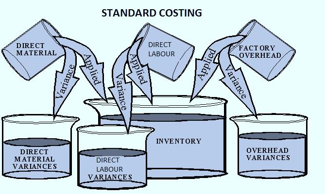
Materials

In manufacturing company, materials and labour are the most important factors for the production.

Raw materials are converted into semi-finished goods and finished goods with the help of labour.

While manufacturing the goods, all the input goods are NOT output or yield.

There are normal and abnormal losses.

When the company cannot stop or control loss of goods in natural basis; it is called normal loss.

Normal losses are weight loss, shrinkage, evaporation, rust etc.

When the company can stop or control loss but could not control, it is known as abnormal loss.

Abnormal loss is due to carelessness, fatigue, rough handling, abnormal or bad working condition, lack of proper knowledge, low quality raw materials, machine break down, accident etc.

We will study following materials variances in this topic:

Materials cost variance

Materials price variance

Materials usage variance

Materials mix variance

Materials yield variance

Click on the photo for FREE eBooks

Labour

In every manufacturing company and business organization needs human being resources.

These human beings may be the resource of administrators and labour.

Without labour, a manufacturing company cannot complete its production.

It is saying, “Talented, caliber and skilled manpower is the other assets of the business organization.”

There are three types of labour.

They are unskilled labour, semi-skilled labour and skilled labour.

Unskilled labour gets fewer wages but skilled labour gets the highest wages.

The payment made to the labour in exchange for its service is called labour cost.

It is a major part of the total cost of production.

Labour cost is also commonly called wages.

Labour cost or wages is one of the major elements of cost.

Labour cost represents the expense incurred on both direct and indirect labour.

Unproductive time is known as idle time.

It may be due to normal or abnormal reasons.

In idle time, workers have been paid without any production activity.

To identify the reasons for the idle time in the factory, an idle time card is maintained.

We will study following labour variances in this topic:

Labour rate variance

Labour efficiency variance

Labour idle time variance

Labour mix variance

Labour yield variance

Labour cost variance

Keep In Mind (KIM)

Cost variance	Overhead cost variance (OCV):
Materials cost variance (MCV)	Three overhead variances are:
Labour cost variance (LCV)	Spending variance (SV)
Overhead cost variance (OCV)	Efficiency variance (EV)
	Capacity variance (CV)

Materials variance (MCV)	Labour variances
Materials cost variance (MCV)	Labour rate variance (LRV)
Materials price variance (MPV)	Labour efficiency variance (LEV)
Materials usage variance (MUV)	Labour idle time variance (LITV)
Materials mix variance (MMV)	Labour mix variance (LMV)
Materials yield variance (MYV)	Labour yield variance (LYV)
	Labour cost variance (LCV)

Preliminaries to Established Standard Costing

Standard costing is very effective tool to control element of cost like direct cost and overhead.

The following preliminaries should be established:

Establishment of cost center

Types of standard

Setting the standard

Establishment of Cost Center

Cost center is a location, person or item of equipment that ascertains or uses for the purpose of cost control.

Establishment of cost centers is necessary for fixing responsibilities.

The main objectives of cost account are:

Who or which department will do the work.

Who or which department will do the expenses.

Who or which department will control unfavourable variances.

Who or which department will bills receivable responsible etc.

Types of Standards

Current standard

The standard fixed for short period is known as current standard.

It reflects the work performance.

It is not suitable for long period.

Generally, it is based on one accounting year period.

Ideal or perfect standard

It presents high level of efficiency.

Under this, everything should be perfect.

Such as best quality materials, expert labour, modern technology machines, time management, minimum loss of materials etc.

It is only hypothesis or theory.

It is not realistic and practicable.

Expected standard

It is based on past performance and present condition.

It is prepared for future but based on present.

If there is any changing in planning, it is modified.

Basic standard

If standard is maintained for long time, it is called basic standard.

These standards are revised only in changing of materials and technology.

Basic standard can’t serve for cost control because it is not revised for long time.

Normal or average standard

It is based on one trade circle.

Generally, trade circle is 7 to 10 years.

It may be difference than actual because it is based on average as well as for long time.

Setting the Standard

There are various types of standards.

Out of them, some important standard are direct materials, direct labour and direct overhead.

Direct material

Products are made by raw materials.

Raw materials are called direct materials.

Direct materials are based on standard quantity and standard rate.

While producing the goods, not only quantity is fixed but also rate of materials are fixed.

Direct labour

Under direct labour, standard time and standard wages are fixed.

Then time and motion study is analyzed.

Time can be fixed from past data.

Direct overhead

Under overhead, all the expenses except direct material and direct wages are included.

Differences between Standard Costing and Budgetary Control

Both standard costing and budgetary control have same objectives of maximum efficiency and cost reduction.

It is possible by pre-determined standard and comparison with actual cost.

Although both are useful tools for management yet there are some differences.

Differences between Standard Costing and Budgetary Control

Bases	Standard Costing	Budgetary Control
Based	Standard costing is based on technical assessment.	Budgetary control can be prepared on the basis of past figures adjusted to future trends.
Covering	It fulfills various product costing or element of cost only.	It covers production, sales, purchase, cash, income, expenditures etc.
Applicable	It is applicable to manufacturing company, production or service.	It is applicable almost all business organizations.
Depends	It is based on budgetary control. In the absence of budgetary control, standard costing cannot exist.	Budgetary control has separate existence; It is not based on standard costing.
Total or per unit	Standard costing works on per unit of production or service.	Budgetary control works on specific period with total amount.

Advantages of Standard Costing

The main advantage of standard costing are:

The main objective of standard costing is to know perform evaluation established by management.

It minimizes the wastage by detecting variances and suggests to correction.

Under standard costing, cost centers are established.

The related cost department and persons are responsible for cost control.

Standard costing encourages to control unfavourable variances.

It helps to management attention toward not proceeding according to plan.

It is effective tool for business planning, budgeting, marginal costing, inventory valuation etc.

It provides a basis for incentive wage scheme to workers and supervisors etc.

Limitation or Disadvantages of Standard Costing

The main disadvantage of standard costing are:

Standard costing system is not suitable for small industries because it needs high degree skill and cost.

It controls the operating part of organization but it ignores other items like quality, lead time, service, customer satisfaction etc.

It is useless where ‘just in time’ principle is adopted.

It may not be very effective where non-standard products are manufactured or service rendered.

Variance Analysis

Difference between planned cost and actual cost is variance.

If actual cost is less than planned, it is favorable variance.

On the contrary, if actual cost is more than planned, it is unfavorable variance.

EP Online Study

Thank you for investing your time.

Please comment on the article.

You can help us by sharing this post on your social media platform.

Jay Google, Jay YouTube, Jay Social Media

जय गूगल. जय युट्युब, जय सोशल मीडिया

The post Standard Costing | Types of Standards | Standard Costing vs Budgetary Control appeared first on EP Online Study.